Coursera Week 2 - Linear Regression with Multiple Variables
coursera week 2 - linear regression with multiple variables 1
1. Multiple Features
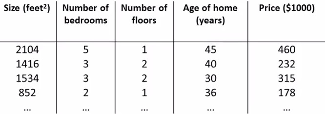
\begin{align}x_j^{(i)} &= \text{value of feature } j \text{ in the }i^{th}\text{ training example} \newline x^{(i)}& = \text{the column vector of all the feature inputs of the }i^{th}\text{ training example} \newline m &= \text{the number of training examples} \newline n &= \left| x^{(i)} \right| ; \text{(the number of features)} \end{align}
Macdown Version 0.6.4 (786) MathJax the same this web
1.1 hypothesis function
Now define the multivariable form of the hypothesis function as follows, accommodating these multiple features:
multivariable hypothesis function
Using the definition of matrix multiplication, our multivariable hypothesis function can be concisely represented as:
\begin{align} h_\theta(x) =\begin{bmatrix}\theta_0 \hspace{2em} \theta_1 \hspace{2em} ... \hspace{2em} \theta_n\end{bmatrix}\begin{bmatrix}x_0 \newline x_1 \newline \vdots \newline x_n\end{bmatrix}= \theta^T x \end{align}
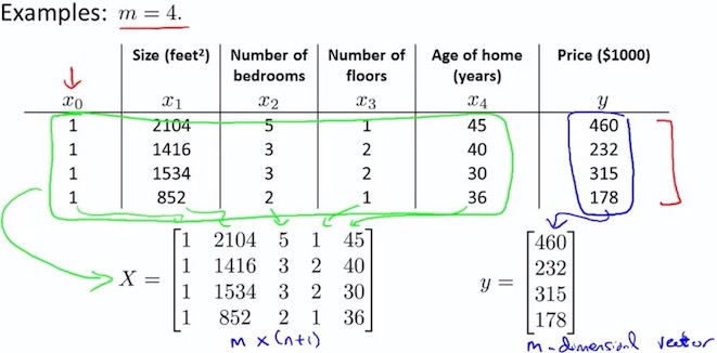
The training examples are stored in X row-wise, like such:
\begin{align} X = \begin{bmatrix}x^{(1)}_0 & x^{(1)}\_1 \newline x^{(2)}_0 & x^{(2)}\_1 \newline x^{(3)}\_0 & x^{(3)}\_1 \end{bmatrix}&,\theta = \begin{bmatrix}\theta\_0 \newline \theta\_1 \newline \end{bmatrix} \end{align}
You can calculate the hypothesis as a column vector of size (m x 1) with:
For the rest of these notes, X will represent a matrix of training examples
2. Cost function
For the parameter vector θ (of type or in , the cost function is:
The vectorized version is:
vectorized version is very good!
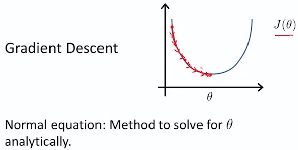
3. Gradient Desc Multivariable
Matrix Notation
The Gradient Descent rule can be expressed as:
Where is a column vector of the form:
The j-th component of the gradient is the summation of the product of two terms:
\begin{align} \; &\frac{\partial J(\theta)}{\partial \theta\_j} &=& \frac{1}{m} \sum\limits\_{i=1}^{m} \left(h\_\theta(x^{(i)}) - y^{(i)} \right) \cdot x\_j^{(i)} \newline \; & &=& \frac{1}{m} \sum\limits\_{i=1}^{m} x\_j^{(i)} \cdot \left(h\_\theta(x^{(i)}) - y^{(i)} \right) \end{align}
在数学中,一个多变量的函数的偏导数是它关于其中一个变量的导数,而保持其他变量恒定。
Sometimes, the summation of the product of two terms can be expressed as the product of two vectors.
\begin{align}\; &\frac{\partial J(\theta)}{\partial \theta\_j} = \frac1m \vec{x\_j}^{T} (X\theta - \vec{y}) \newline &\nabla J(\theta) = \frac 1m X^{T} (X\theta - \vec{y}) \newline \end{align}
Finally, the matrix notation (vectorized) of the Gradient Descent rule is:
The gradient descent equation itself is generally the same form; we just have to repeat it for our ‘n’ features:
\begin{align} & \text{repeat until convergence:} \; \lbrace \newline \; & \theta\_0 := \theta\_0 - \alpha \frac{1}{m} \sum\limits\_{i=1}^{m} (h\_\theta(x^{(i)}) - y^{(i)}) \cdot x\_0^{(i)}\newline \; & \theta\_1 := \theta\_1 - \alpha \frac{1}{m} \sum\limits\_{i=1}^{m} (h\_\theta(x^{(i)}) - y^{(i)}) \cdot x\_1^{(i)} \newline \; & \theta\_2 := \theta\_2 - \alpha \frac{1}{m} \sum\limits\_{i=1}^{m} (h\_\theta(x^{(i)}) - y^{(i)}) \cdot x\_2^{(i)} \newline & \cdots \newline \rbrace \end{align}
In other words:
\begin{align} & \text{repeat until convergence:} \; \lbrace \newline \; & \theta\_j := \theta\_j - \alpha \frac{1}{m} \sum\limits\_{i=1}^{m} (h\_\theta(x^{(i)}) - y^{(i)}) \cdot x\_j^{(i)} \; & \text{for j := 0..n} \newline \rbrace \end{align}
3.1 Feature Scaling
Idea : Make sure features are on a similar scale 特征缩放
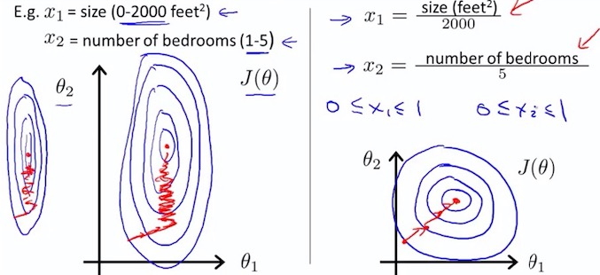
Get every feature into approximately a range.
Replace with to make features have approximately zero mean (Do not apply to = 1).
如果多个特征值,大多处在一个相近的范围,梯度下降就能更快的收敛。
因为 2000/5 比较大,所以轮廓图,使得椭圆更加的瘦长,好比 收敛的更慢。
3.2 learning rate
\begin{align} \theta\_j := \theta\_j - \alpha \frac{\partial}{\partial \theta\_j} J(\theta) \end{align}
- Debugging : How to make sure gradient descent is working correctly
- How to choose learning rate
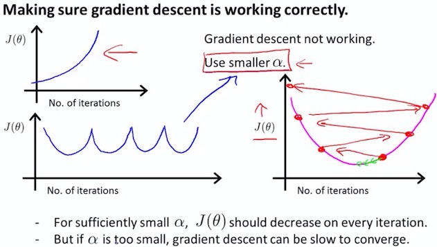
Summary
- if is too small: slow convergence [kən’vɜːdʒəns] 收敛
- if is too large: may not decrease on every iteration; may not converge.
To choose , try
…, 0.001, 0.01, 0.1, 1, …
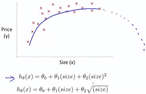
4. Polynomial Regression
4.1 Polynomial Regression
![Polynomial [,pɒlɪ'nəʊmɪəl]](/images/ml/coursera/ml-ng-w2-05.png)
Feature normalization is very important
4.2 Choice of features
@2017-02-10 review done
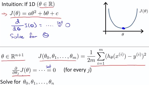
5. Normal Equation
5.1 num and vector
\begin{align}\; &\frac{\partial J(\theta)}{\partial \theta\_j} = \frac1m \vec{x\_j}^{T} (X\theta - \vec{y}) \newline &\nabla J(\theta) = \frac 1m X^{T} (X\theta - \vec{y}) \newline \end{align}
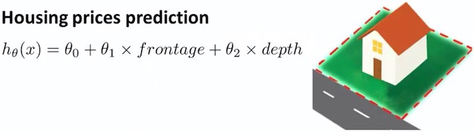
5.2 house price example
\begin{align} \nabla J(\theta) = \frac 1m X^{T} (X\theta - \vec{y}) \newline \end{align}
令 $\nabla J(\theta) = 0 $
So, $\theta = (X^T X){-1}XT y $
5.3 training, features
| Gradient Descent | Normal Equation |
|---|---|
| Need to choose | No need to choose |
| Needs many iterations | Don’t need to iterate |
| Works well even when is large | Slow if is very large |
it is usually around ten thousand that I might start to consider switching over to gradient descents or maybe, some other algorithms that we’ll talk about later in this class
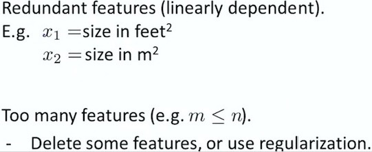
5.4 is non-invertible
$\theta = (X^T X){-1}XT y $
What is non-invertible? (singular / degenerate)
When is non-invertible, this is very few.
What is non-invertible?
Checking if Disqus is accessible...