import numpy as np
np.random.seed(1337)  # for reproducibility
from keras.models import Sequential
from keras.layers import Dense
import matplotlib.pyplot as plt # 可视化模块

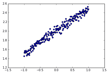
# create some data
X = np.linspace(-1, 1, 200)

np.random.shuffle(X)    # randomize the data

Y = 0.5 * X + 2 + np.random.normal(0, 0.05, (200, ))

# plot data
plt.scatter(X, Y)
plt.show()

X_train, Y_train = X[:160], Y[:160]     # train 前 160 data points
X_test, Y_test = X[160:], Y[160:]       # test 后 40 data points

model = Sequential()
model.add(Dense(output_dim=1, input_dim=1))

# choose loss function and optimizing method
model.compile(loss='mse', optimizer='sgd')

# mse 均方误差； optimizer sgd 随机梯度下降法.

# training
print('Training -----------')
for step in range(301):
    cost = model.train_on_batch(X_train, Y_train)
    if step % 100 == 0:
        print('train cost: ', cost)

"""
Training -----------
train cost:  4.111329555511475
train cost:  0.08777070790529251
train cost:  0.007415373809635639
train cost:  0.003544030711054802
"""

# test
print('\nTesting ------------')
cost = model.evaluate(X_test, Y_test, batch_size=40)
print('test cost:', cost)
W, b = model.layers[0].get_weights()
print('Weights=', W, '\nbiases=', b)

"""
Testing ------------
40/40 [==============================] - 0s
test cost: 0.004269329831
Weights= [[ 0.54246825]] 
biases= [ 2.00056005]
"""

# plotting the prediction
Y_pred = model.predict(X_test)
plt.scatter(X_test, Y_test)
plt.plot(X_test, Y_pred)
plt.show()

numpy.random.normal(loc=0.0, scale=1.0, size=None)