官方给出的例子,用多层 LSTM 来实现 PTBModel 语言模型,比如: tensorflow笔记:多层LSTM代码分析 感觉这些例子还是太复杂了,所以这里写了个比较简单的版本
声明: 本文部分内容转自 永永夜 Tensorflow学习之路
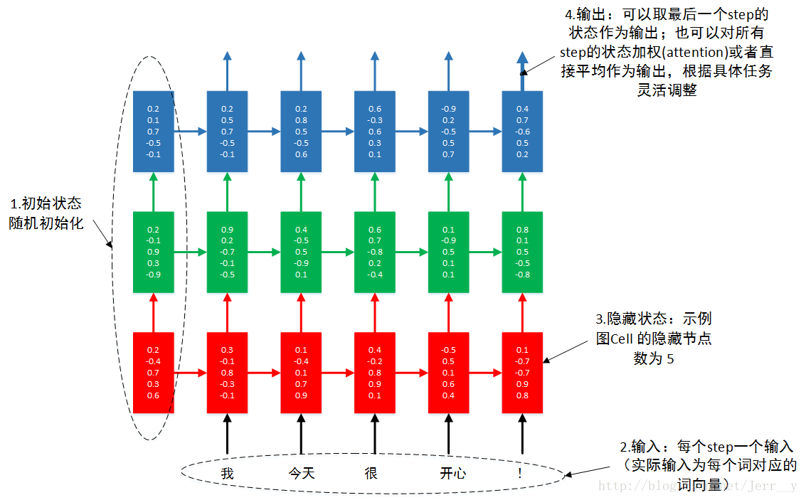
自己做了一个示意图,希望帮助初学者更好地理解 多层RNN.
通过本例,你可以了解到单层 LSTM 的实现,多层 LSTM 的实现。输入输出数据的格式。 RNN 的 dropout layer 的实现。
准备数据
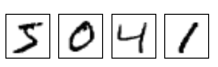
MNIST 是在机器学习领域中的一个经典问题。该问题解决的是把 28x28像素 的灰度手写数字图片识别为相应的数字,其中数字的范围从 0到9.
MNIST 数据集 包含了 60000 张图片来作为训练数据,10000 张图片作为测试数据。每张图片都代表了 0~9 中的一个数字。图片大小都为 28*28,处理后的每张图片是一个长度为 784 的一维数组,这个数组中的元素对应图片像素矩阵提供给神经网络的输入层,像素矩阵中元素的取值范围 [0, 1], 它代表了颜色的深浅。其中 0 表示白色背景(background),1 表示黑色前景(foreground)。
1 2 3 4 5 6 7 8 9 10 11 12 13 14 import tensorflow as tfimport numpy as npfrom tensorflow.contrib import rnnfrom tensorflow.examples.tutorials.mnist import input_dataconfig = tf.ConfigProto() config.gpu_options.allow_growth = True sess = tf.Session(config=config) mnist = input_data.read_data_sets('MNIST_data' , one_hot=True ) print (mnist.train.images.shape)
1
2
3
4
5
Extracting MNIST_data/train-images-idx3-ubyte.gz Extracting MNIST_data/train-labels-idx1-ubyte.gz Extracting MNIST_data/t10k-images-idx3-ubyte.gz Extracting MNIST_data/t10k-labels-idx1-ubyte.gz (55000, 784) # 训练集图片 - 55000 张 * 784维一维数组
执行 input_data.read_data_sets 后自动创建一个目录 MNIST_data,并开始下载数据
1
2
3
4
5
6
7
8
9
10
11
12
13
14
15
16
(anaconda3) ➜ ll total 24 drwxr-xr-x 6 blair staff 192B Oct 9 16:14 MNIST_data -rw-r--r-- 1 blair staff 2.3K Oct 9 16:13 simple-lstms.ipynb (anaconda3) ➜ ll MNIST_data total 22672 -rw-r--r-- 1 blair staff 1.6M Oct 9 16:14 t10k-images-idx3-ubyte.gz -rw-r--r-- 1 blair staff 4.4K Oct 9 16:14 t10k-labels-idx1-ubyte.gz -rw-r--r-- 1 blair staff 9.5M Oct 9 16:14 train-images-idx3-ubyte.gz -rw-r--r-- 1 blair staff 28K Oct 9 16:14 train-labels-idx1-ubyte.gz (anaconda3)
文件
内容
train-images-idx3-ubyte.gz
训练集图片 - 55000 张 训练图片, 5000 张 验证图片
train-labels-idx1-ubyte.gz
训练集图片对应的数字标签
t10k-images-idx3-ubyte.gz
测试集图片 - 10000 张 图片
t10k-labels-idx1-ubyte.gz
测试集图片对应的数字标签
1
2
3
4
5
print ('training data shape ' , mnist.train.images.shape)print ('training label shape ' , mnist.train.labels.shape)
1
2
3
4
5
6
7
8
9
10
11
12
13
14
15
16
17
18
19
lr = 1e-3 batch_size = tf.placeholder(tf.int32, []) keep_prob = tf.placeholder(tf.float32, []) input_size = 28 timestep_size = 28 hidden_size = 256 layer_num = 2 class_num = 10 _X = tf.placeholder(tf.float32, [None , 784 ]) y = tf.placeholder(tf.float32, [None , class_num])
1 2 3 4 5 6 7 8 9 10 11 12 13 14 15 16 17 18 19 20 21 22 23 24 25 26 27 28 29 30 31 32 33 34 35 36 37 38 39 40 41 42 43 44 X = tf.reshape(_X, [-1 , 28 , 28 ]) lstm_cell = rnn.BasicLSTMCell(num_units=hidden_size, forget_bias=1.0 , state_is_tuple=True ) lstm_cell = rnn.DropoutWrapper(cell=lstm_cell, input_keep_prob=1.0 , output_keep_prob=keep_prob) mlstm_cell = rnn.MultiRNNCell([lstm_cell] * layer_num, state_is_tuple=True ) init_state = mlstm_cell.zero_state(batch_size, dtype=tf.float32) outputs = list () state = init_state with tf.variable_scope('RNN' ): for timestep in range (timestep_size): if timestep > 0 : tf.get_variable_scope().reuse_variables() (cell_output, state) = mlstm_cell(X[:, timestep, :], state) outputs.append(cell_output) h_state = outputs[-1 ]
1 2 3 4 5 6 7 8 9 10 11 12 13 14 15 16 17 18 19 20 21 22 23 24 25 26 27 28 29 30 31 32 W = tf.Variable(tf.truncated_normal([hidden_size, class_num], stddev=0.1 ), dtype=tf.float32) bias = tf.Variable(tf.constant(0.1 ,shape=[class_num]), dtype=tf.float32) y_pre = tf.nn.softmax(tf.matmul(h_state, W) + bias) cross_entropy = -tf.reduce_mean(y * tf.log(y_pre)) train_op = tf.train.AdamOptimizer(lr).minimize(cross_entropy) correct_prediction = tf.equal(tf.argmax(y_pre,1 ), tf.argmax(y,1 )) accuracy = tf.reduce_mean(tf.cast(correct_prediction, "float" )) sess.run(tf.global_variables_initializer()) for i in range (2000 ): _batch_size = 128 batch = mnist.train.next_batch(_batch_size) sess.run(train_op, feed_dict={_X: batch[0 ], y: batch[1 ], keep_prob: 0.5 , batch_size: _batch_size}) if (i+1 )%200 == 0 : train_accuracy = sess.run(accuracy, feed_dict={ _X:batch[0 ], y: batch[1 ], keep_prob: 1.0 , batch_size: _batch_size}) print "Iter%d, step %d, training accuracy %g" % ( mnist.train.epochs_completed, (i+1 ), train_accuracy) print "test accuracy %g" % sess.run(accuracy, feed_dict={ _X: mnist.test.images, y: mnist.test.labels, keep_prob: 1.0 , batch_size:mnist.test.images.shape[0 ]})
1
2
3
4
5
6
7
8
9
10
11
Iter0, step 200, training accuracy 0.851562 Iter0, step 400, training accuracy 0.960938 Iter1, step 600, training accuracy 0.984375 Iter1, step 800, training accuracy 0.960938 Iter2, step 1000, training accuracy 0.984375 Iter2, step 1200, training accuracy 0.9375 Iter3, step 1400, training accuracy 0.96875 Iter3, step 1600, training accuracy 0.984375 Iter4, step 1800, training accuracy 0.992188 Iter4, step 2000, training accuracy 0.984375 test accuracy 0.9858
我们一共只迭代不到 5 个 epoch,在测试集上就已经达到了 0.98 的准确率,可以看出来 LSTM 在做这个字符分类的任务上还是比较有效的,而且我们最后一次性对 10000 张测试图片进行预测,才占了 725 MiB 的显存。而我们在之前的两层 CNNs 网络中,预测 10000 张图片一共用了 8721 MiB 的显存,差了整整 12 倍呀!! 这主要是因为 RNN/LSTM 网络中,每个时间步所用的权值矩阵都是共享的,可以通过前面介绍的 LSTM 的网络结构分析一下,整个网络的参数非常少。
1
2
3
4
5
6
7
roll_jj: 博主你好, outputs, state = tf.nn.dynamic_rnn(mlstm_cell, inputs=X, initial_state=init_state, time_major=False) h_state = outputs[:, -1, :] 这两句话里,outputs的三个维度是什么意思,为什么把中间那个维度去掉就是我们要的输出结果了?(1年前#6楼)收起回复举报回复 Jerr__y CQU_HYX回复 roll_jj: 是的(1年前) roll_jj roll_jj回复 CQU_HYX: 谢谢博主解答。我看官方的那个PTB例子里,没有取[-1]的这个操作,而是用了output = tf.reshape(tf.concat(1, outputs), [-1, size])操作,这是因为预测目标的不同么?(1年前) Jerr__y CQU_HYX回复 roll_jj: 原文注释上面有说了,outputs.shape = [batch_size, timestep_size, hidden_size]。 因为是分类问题,所有只需要在看完最后一行像素后才输出分类结果。-1 表示取最后一个 timestep 的结果, 而不是说把中间维度去掉
Checking if Disqus is accessible...