Neural Networks and Deep Learning (week3) - Shallow Neural Networks

blairchen

data-science

Publish：Jul 14, 2018

views

正式进入神经网络的学习. 当然, 我们先从简单的只有一个隐藏层的神经网络开始。

在学习完本周内容之后, 我们将会使用 Python 实现一个单个隐藏层的神经网络。

1. 常用符号与基本概念

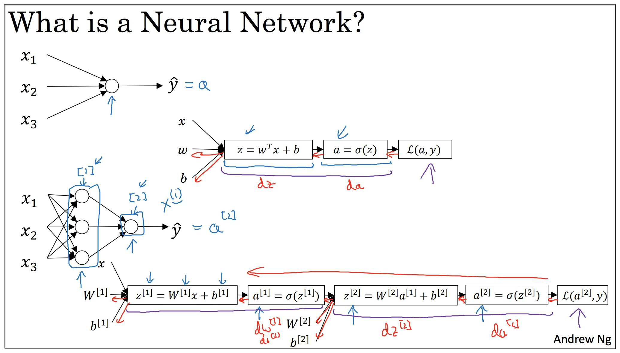
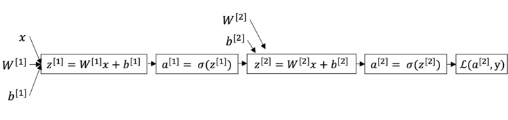
该神经网络完全可以使用上一周所讲的计算图来表示, 和 $LR$ 计算图的区别仅仅在于多了一个 $z$ 和 $a$ 的计算而已.

如果你已经完全掌握了上一周的内容, 那么其实你已经知道了神经网络的前向传播, 反向传播(梯度计算)等等.

要注意的是各种参数, 中间变量 $(a, z)$ 的维度问题. 关于神经网络的基本概念, 这里就不赘述了. 见下图回顾一下:

2. 神经网络中的前向传播

我们先以一个训练样本来看神经网络中的前向传播.
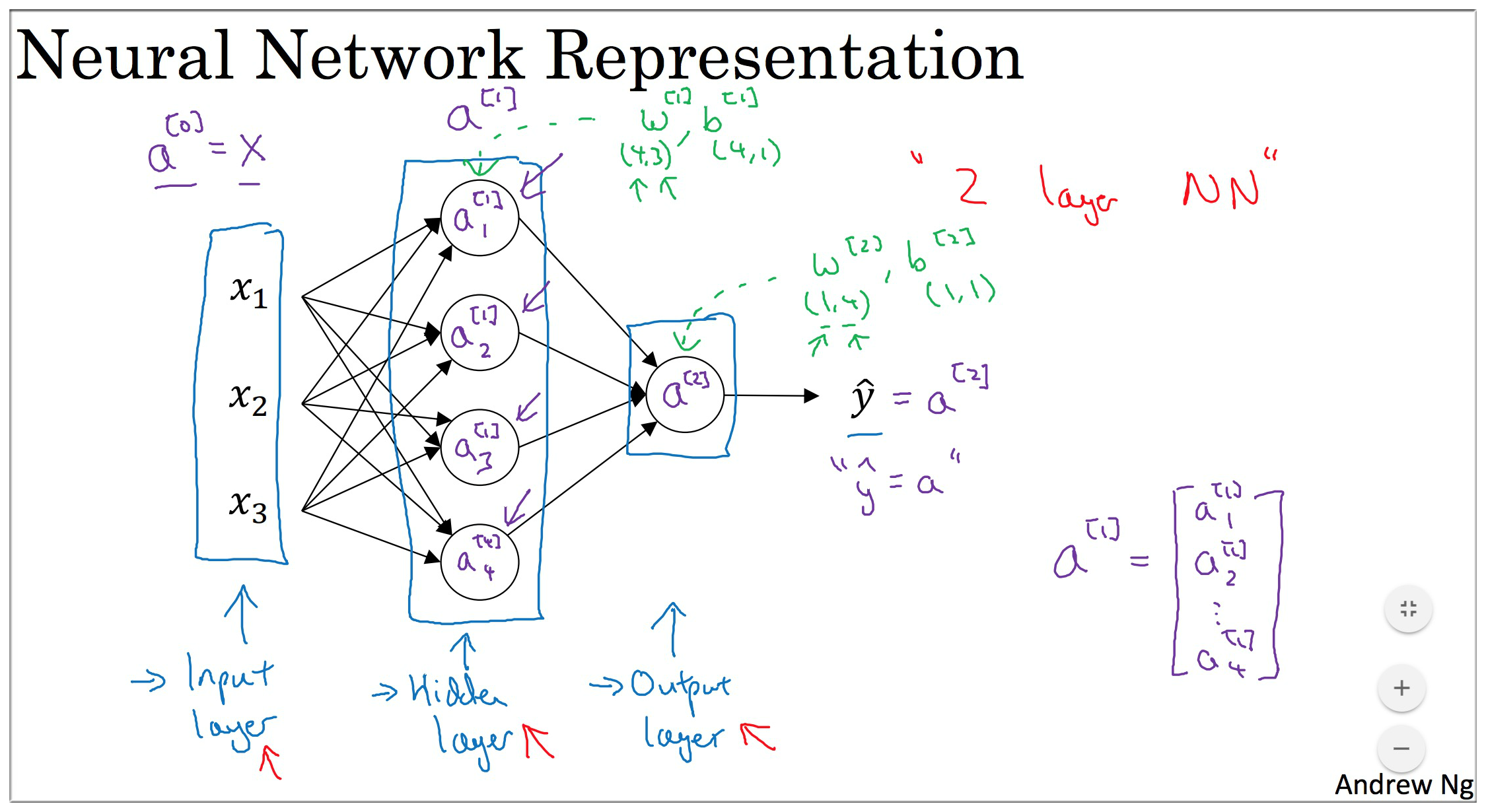
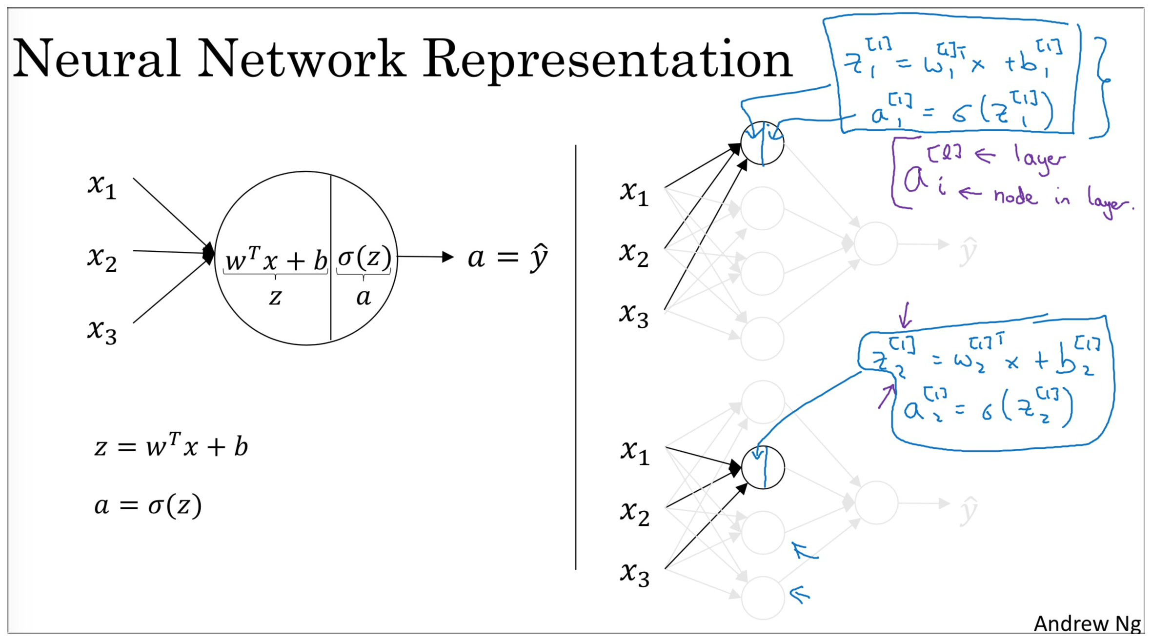
我们只看这个神经网络中的输入层和隐藏层的第一个激活单元(如下图右边所示). 其实这就是一个Logistic Regression.

神经网络中输入层和隐藏层 (不看输出层), 这就不就是四个LR放在一起吗?

在 LR 中 $z$ 和 $a$ 的计算我们已经掌握了, 那么在神经网络中 $z$ 和 $a$ 又是什么呢?

我们记隐藏层第一个 $z$ 为 $z\_1$ , 第二个 $z$ 记为 $z\_2$ 以此类推.
只要将这四个 $z$ 纵向叠加在一起称为一个**列向量 即可得到神经网络中这一层的 $z$ ** ( $a$ 同理).

那么这一层的 $w, b$ 又是如何得到的? 别忘了, 对于参数 $w$ 来说, 它本身就是一个列项量, 那么它是如何做纵向叠加的呢? 我们只需要将其转置变成一个横向量, 再纵向叠加即可.

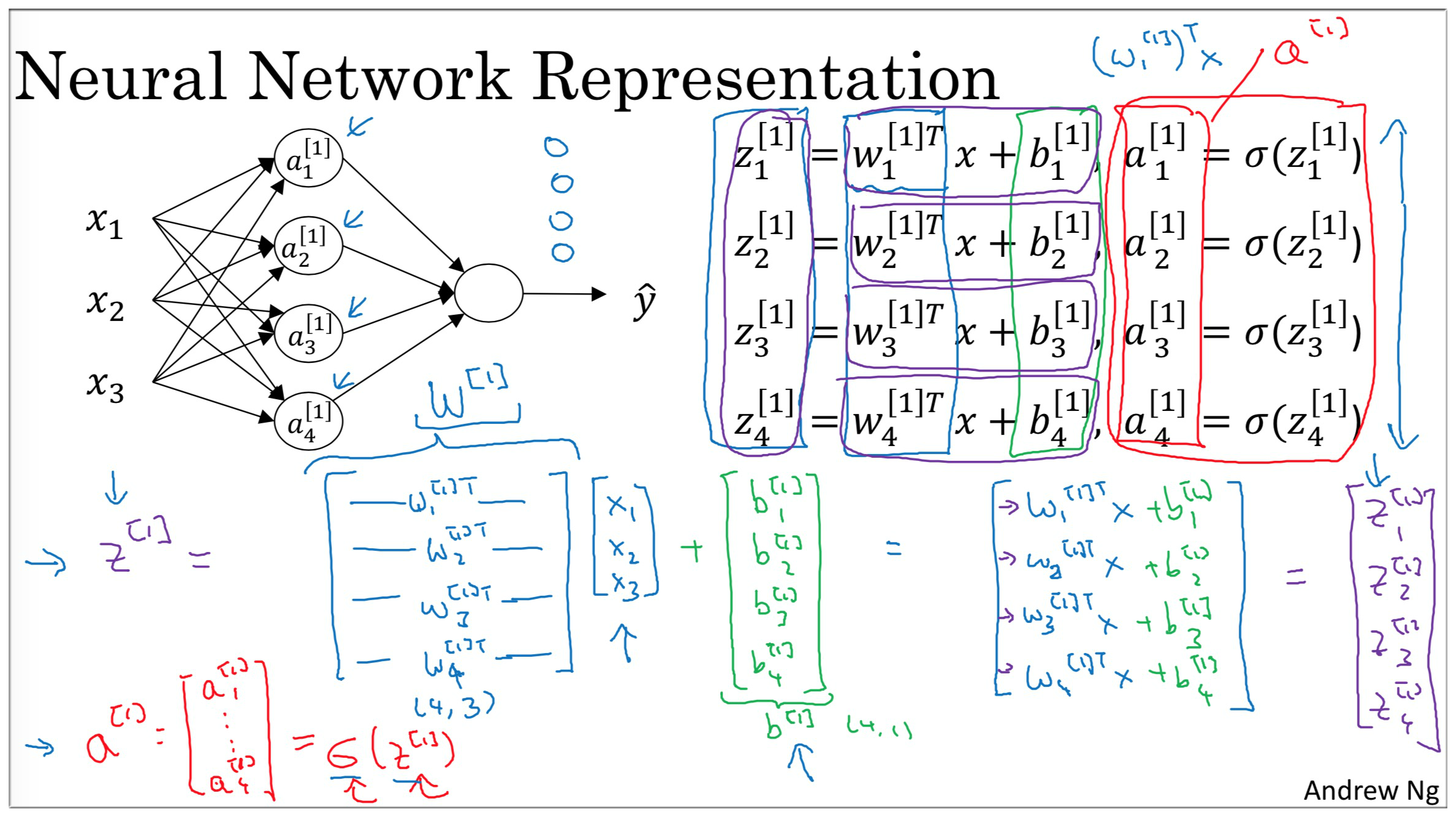
得到隐藏层的 $a$ 之后, 我们可以将其视为输入, 现只看神经网络的隐藏层和输出层, 我们发现这不就是个 $LR$ 嘛.

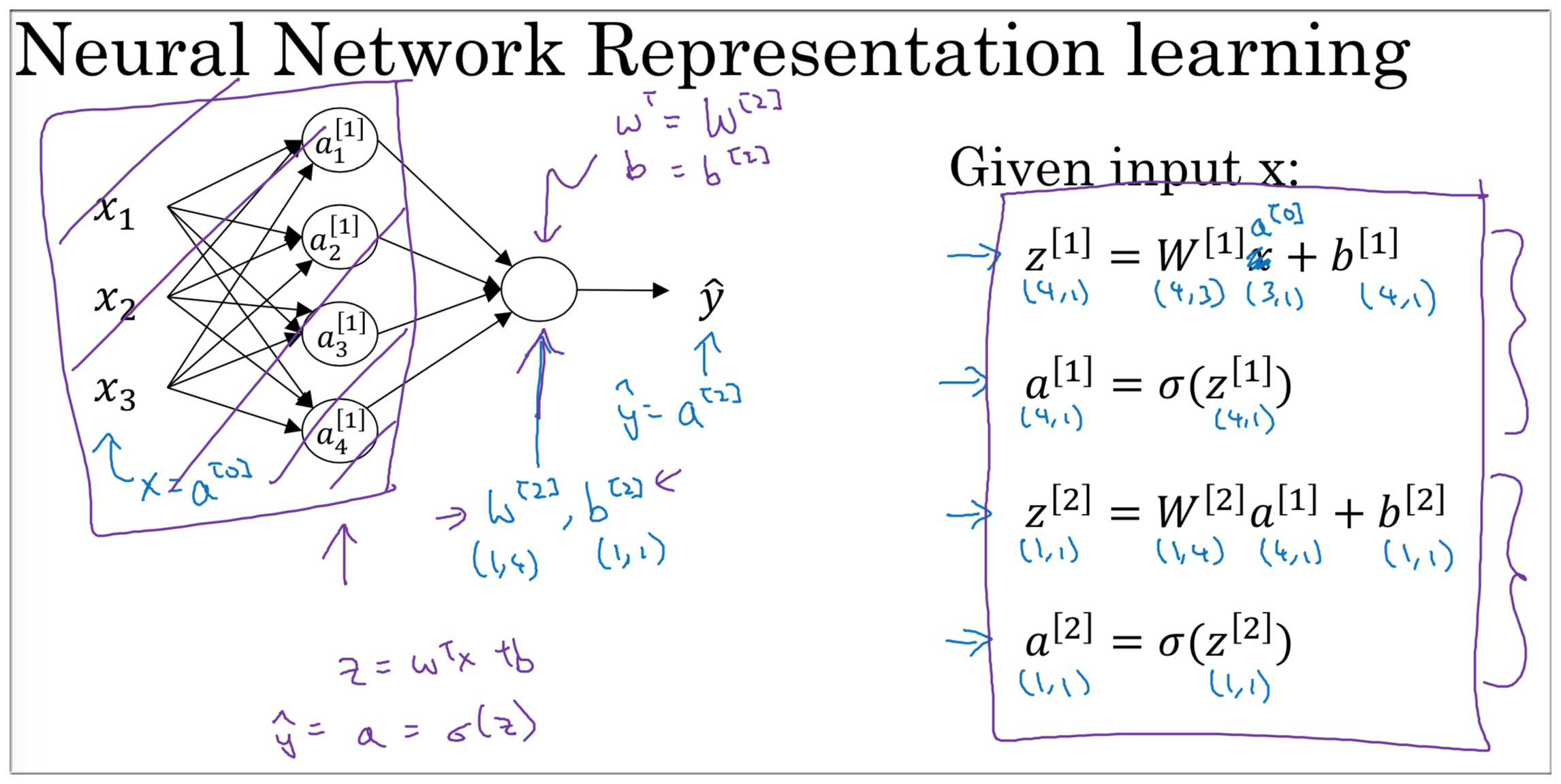
这里总结一下各种变量的维度 (注意: 这里是针对一个训练样本来说的, $n\_L$ 代表的 $L$ 层的节点个数):

$w.shape : (n\_L, n\_{(L-1)})$
$b.shape : (n\_L, 1)$
$z.shape : (n\_L, 1)$
$a.shape : (n\_L, 1)$

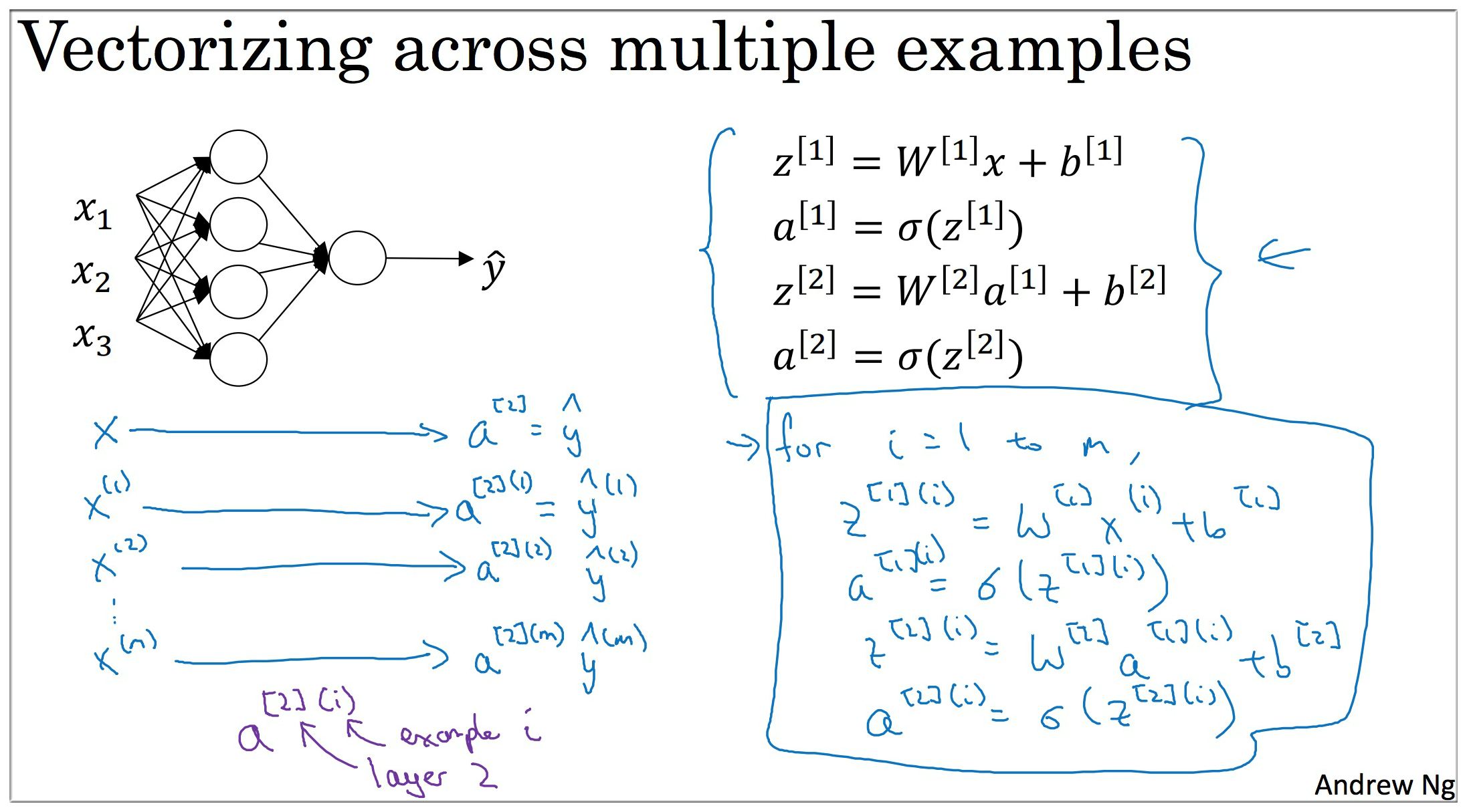
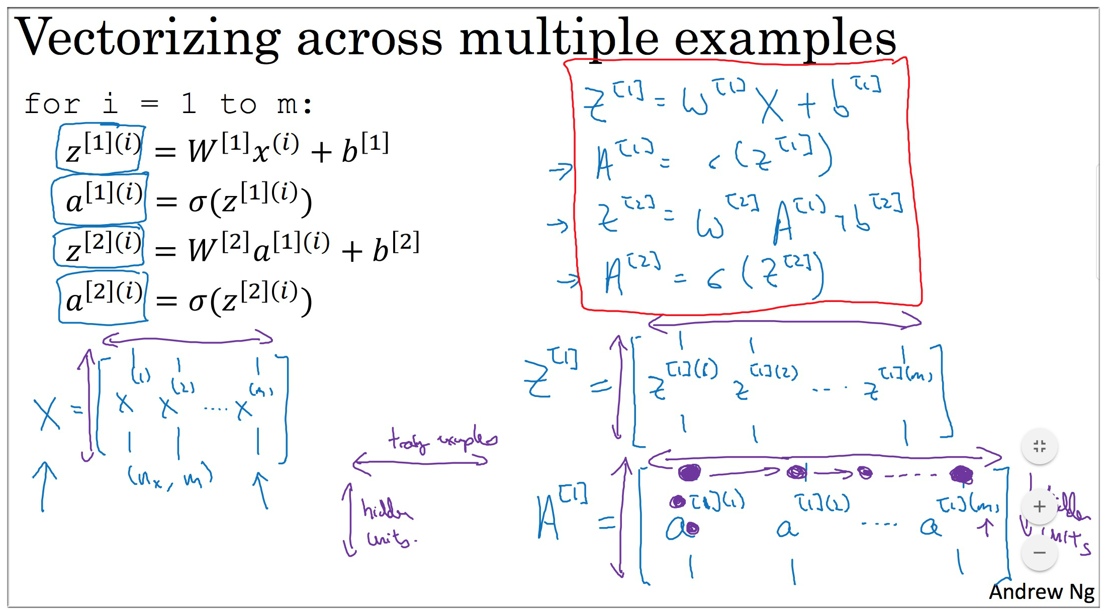
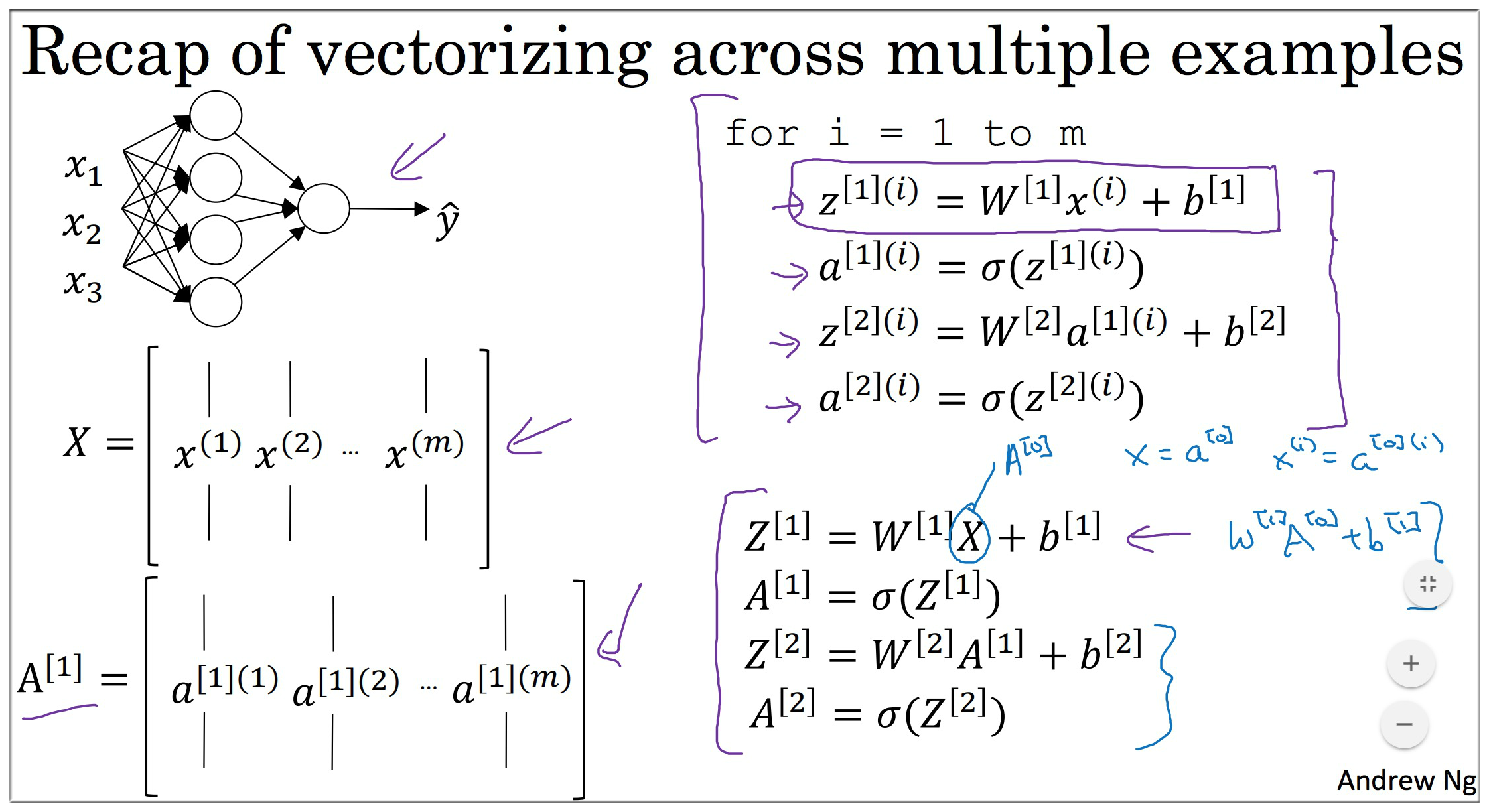
那么如果有 $m$ 个训练样本这些变量的维度又是怎样的呢. 我们思考哪些变量的维度会随着样本数的变化而变化. $w$ 是参数显然它的维度是不会变的. 而输入每一个样本都会有一个 $z$ 和 $a$ , 还记得 $X$ 的形式吗? 同样地, $Z$ 就是将每个样本算出来的 $z$ 横向叠加(A同理). 具体计算过程如下图:

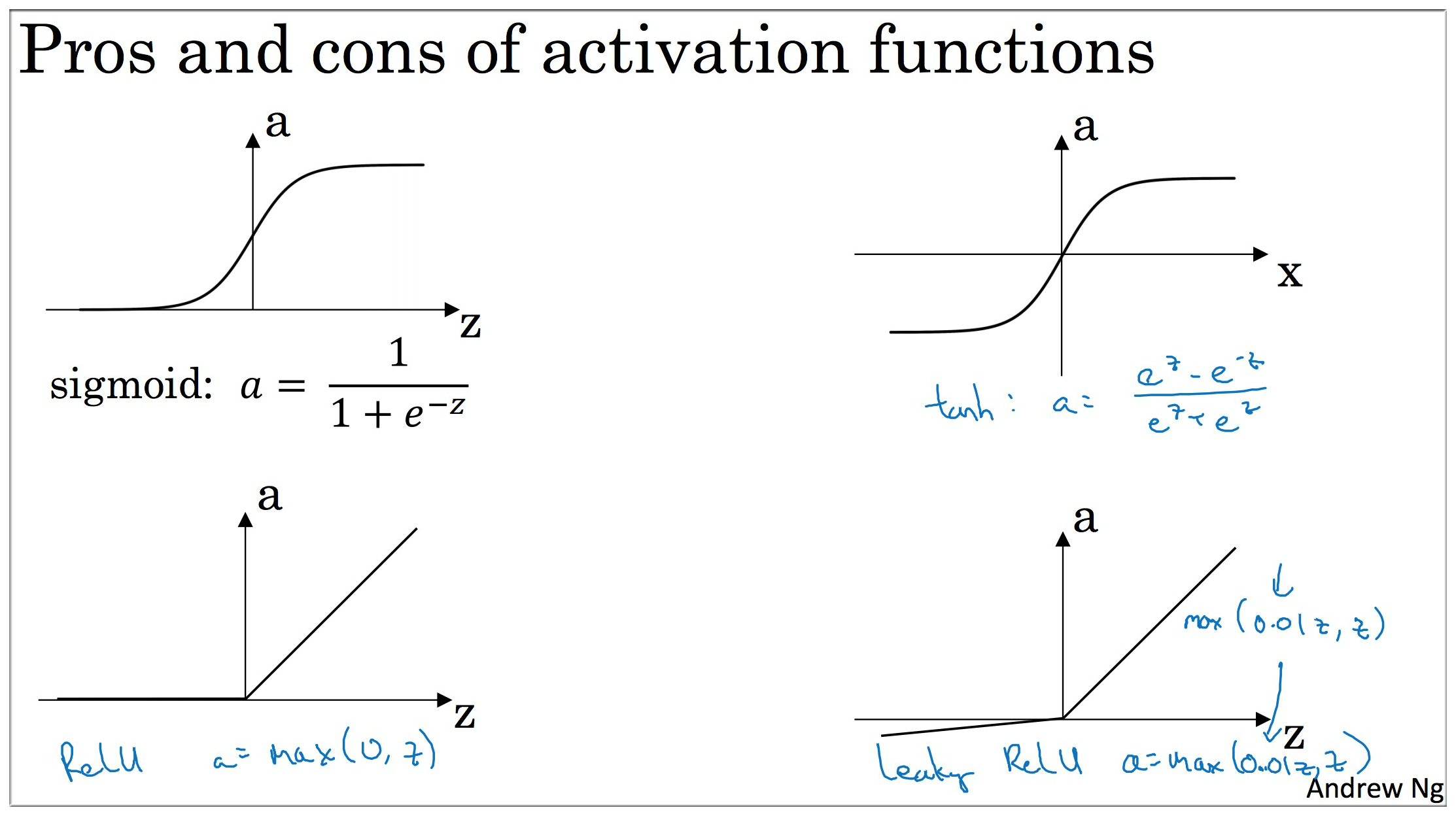
3. 神经网络中的激活函数

四种常用的激活函数: Sigmoid, Tanh, ReLU, Leaky ReLU.

其中 sigmoid 我们已经见过了, 它的输出可以看成一个概率值, 往往用在输出层. 对于中间层来说, 往往是ReLU的效果最好.

Tanh 数据平均值为 0，具有数据中心化的效果，几乎在任何场合都优于 Sigmoid

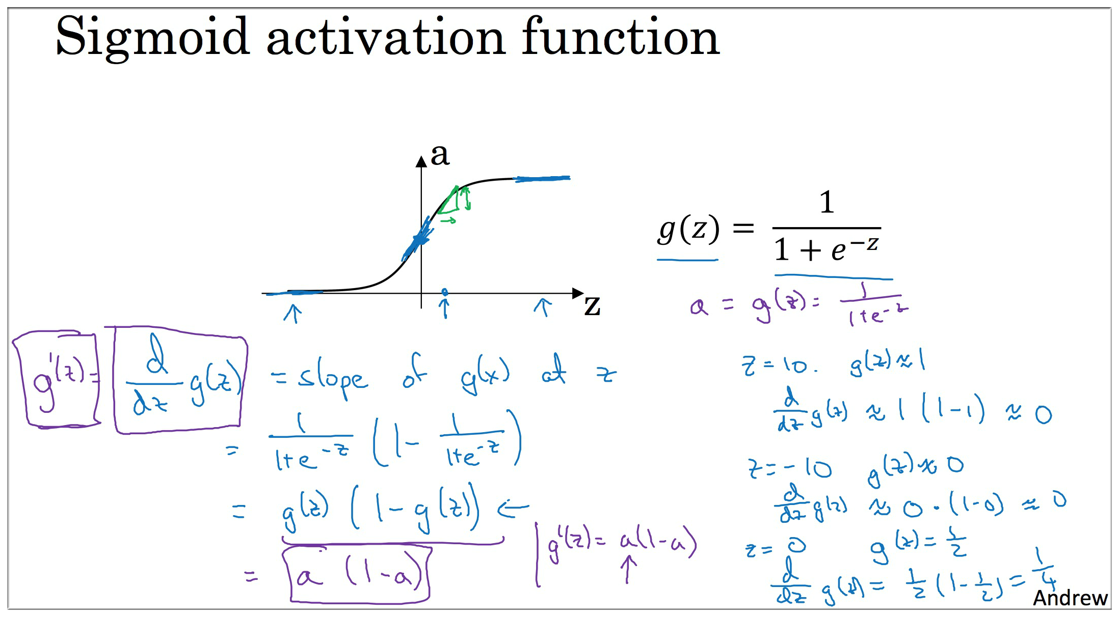
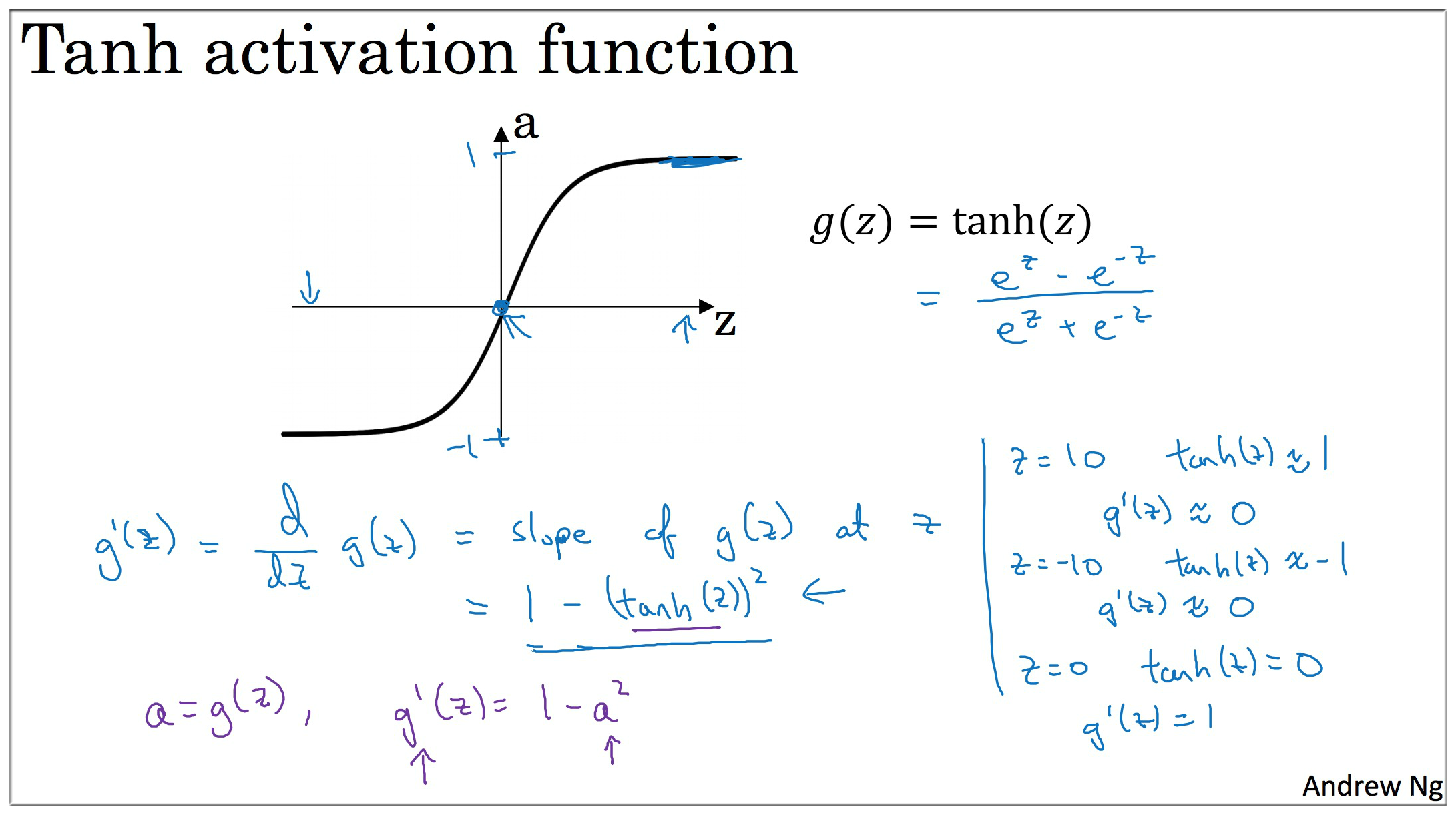
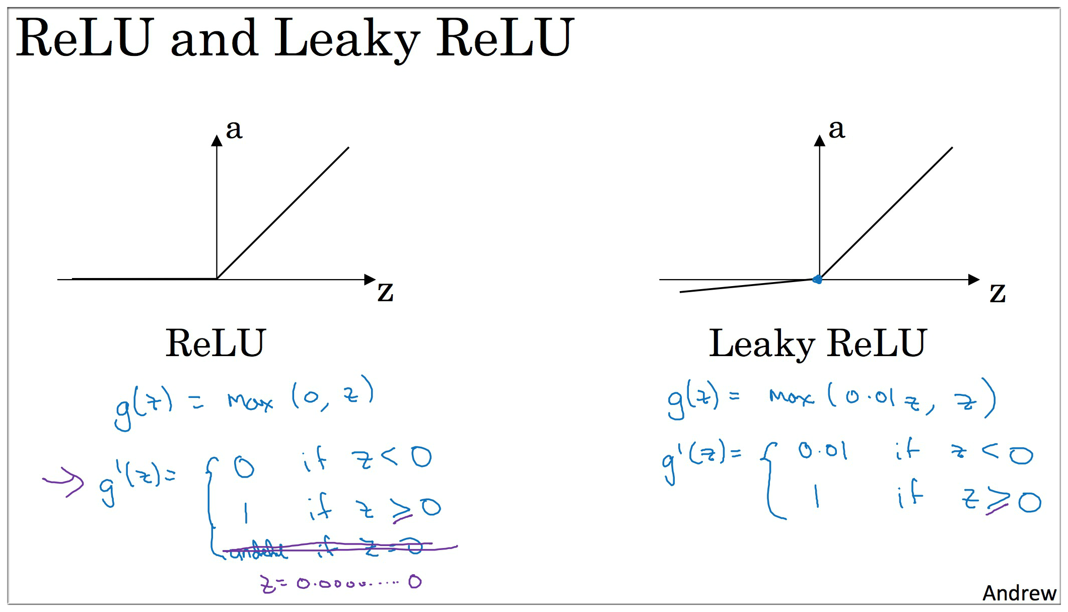
以上激活函数的导数请自行在草稿纸上推导.

derivative of sigmoid activation function

derivative of tanh activation function

derivative of ReLU and Leaky ReLU activation function

为什么需要激活函数? 如果没有激活函数, 那么不论多少层的神经网络都只相当于一个LR. 证明如下:

it turns out that if you use a linear activation function or alternatively if you don’t have an activation function, then no matter how many layers your neural network has, always doing just computing a linear activation function, so you might as well not have any hidden layers.

so unless you throw a non-linearity in there, then you’re not computing more interesting functions.

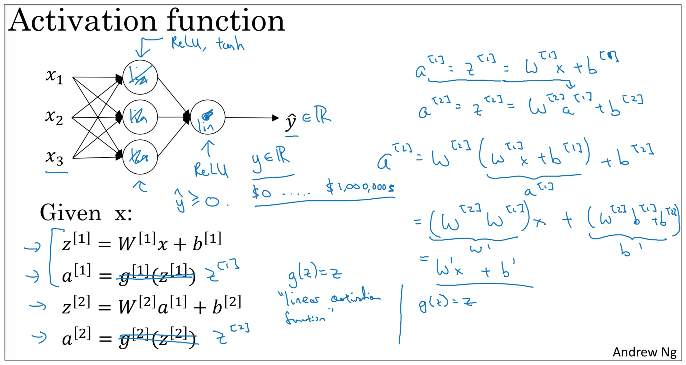
你可以在隐藏层用 tanh，输出层用 sigmoid，说明不同层的激活函数可以不一样。

现实情况是 : the tanh is pretty much stricly superior. never use sigmoid

ReLU (rectified linear unit 矫正线性单元)

tanh 和 sigmoid 都有一个缺点，就是 z 非常大或者非常小，函数的斜率(导数梯度)就会非常小, 梯度下降很慢.

the slope of the function you know ends up being close to zero, and so this can slow down gradient descent

ReLU (rectified linear unit) is well, z = 0 的时候，你可以给导数赋值为 0 or 1，虽然这个点是不可微的. 但实现没有影响.

虽然 z < 0, 的时候，斜率为0，但在实践中，有足够多的隐藏单元令 z > 0, 对大多数训练样本来说是很快的.

Notes:

so the one place you might use as linear activation function, others usually in the output layer.

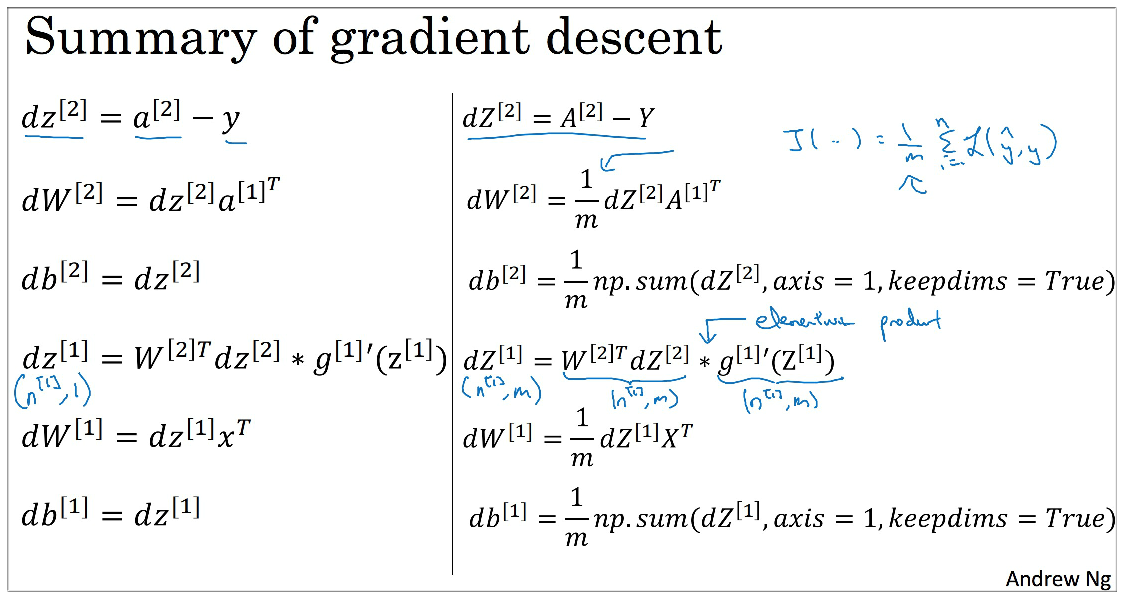
4. 神经网络中的反向传播 back propagation

反向传播最主要的就是计算梯度, 在上一周的内容中, 我们已经知道了LR梯度的计算.

同样的方式, 我们使用计算图来计算神经网络中的各种梯度.

dz^{\[2\]} = \frac{dL}{dz}= \frac{dL}{da^{\[2\]}}\frac{da^{\[2\]}}{dz^{\[2\]}}=a^{\[2\]}-y

dW^{\[2\]}=\frac{dL}{dW^{\[2\]}}=\frac{dL}{dz^{\[2\]}}\frac{dz^{\[2\]}}{dW^{\[2\]}}=dz^{\[2\]}a^{\[1\]}

db^{\[2\]}=\frac{dL}{db^{\[2\]}}=\frac{dL}{dz^{\[2\]}}\frac{dz^{\[2\]}}{db^{\[2\]}}=dz^{\[2\]}

backward propagation :

dz^{\[1\]} = \frac{dL}{dz^{\[2\]}}\frac{dz^{\[2\]}}{da^{\[1\]}}\frac{da^{\[1\]}}{dz^{\[1\]}}=W^{\[2\]T}dz^{\[2\]}*g^{\[1\]’}(z^{\[1\]})

dW^{\[1\]}=\frac{dL}{dW^{\[1\]}}=\frac{dL}{dz^{\[1\]}}\frac{dz^{\[1\]}}{dW^{\[1\]}}=dz^{\[1\]}x^T

db^{\[1\]}=\frac{dL}{db^{\[1\]}}=\frac{dL}{dz^{\[1\]}}\frac{dz^{\[1\]}}{db^{\[1\]}}=dz^{\[1\]}

Notes: $\frac{dL}{dz^{\[2\]}} = dz^{\[2\]}$ ， $\frac{dz^{\[2\]}}{da^{\[1\]}} = W^{\[2\]}$ ， $\frac{da^{\[1\]}}{dz^{\[1\]}}=g^{\[1\]’}(z^{\[1\]})$

下图右边为在 $m$ 个训练样本上的向量化表达:

Notes:

$n^\[0\]$ = input features

$n^\[1\]$ = hidden units

$n^\[2\]$ = output units

5. 神经网络中的参数初始化

在 LR 中我们的参数 $w$ 初始化为 0, 如果在神经网络中也是用相同的初始化, 那么一个隐藏层的每个节点都是相同的, 不论迭代多少次. 这显然是不合理的, 所以我们应该 随机地初始化 $w$ 从而解决这个 sysmmetry breaking problem. 破坏对称问题

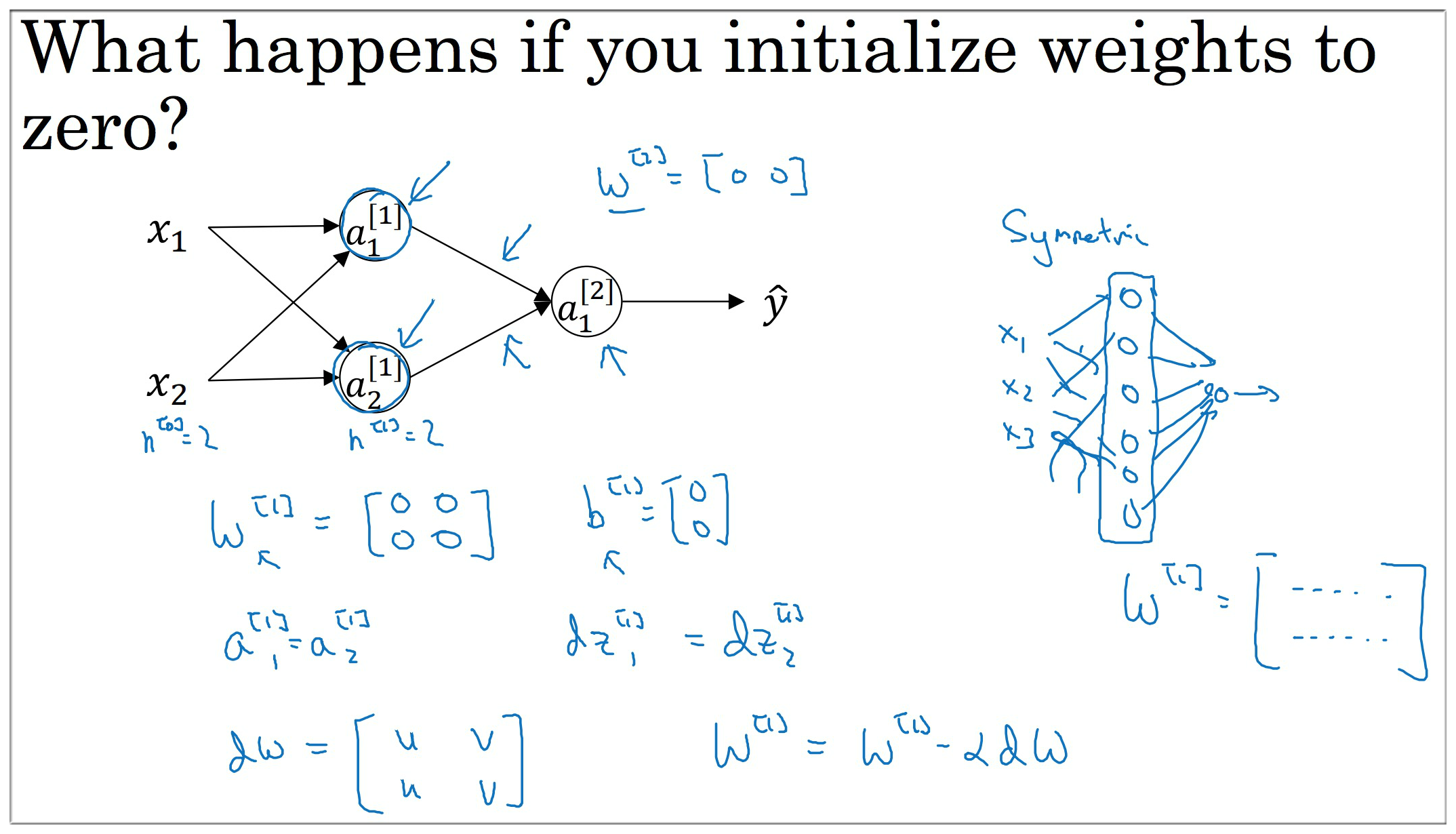
具体初始化代码可参见下图, 其中 乘以 0.01 是为了让参数 $w$ 较小, 加速梯度下降

如激活函数为 tanh 时, 若参数较大则 $z$ 也较大, 此时的梯度接近于 0, 更新缓慢. 如不是 tanh or sigmoid 则问题不大.

this is a relatively shallow neural network without too many hidden layers, so 0.01 maybe work ok.

finally it turns out that sometimes there can be better constants than 0.01.

$b$ 并没有这个 sysmmetry breaking problem, 所以可以 $np.zeros((2, 1))$

6. 用Python搭建简单神经网络

使用Python+Numpy实现一个简单的神经网络. 以下为参考代码

SimpleNeuralNetwork.py

def sigmoid(z):
    return 1. / (1.+np.exp(-z))

class SimpleNeuralNetwork():
    # simple neural network with one hidden layer
    def __init__(self, input_size, hidden_layer_size):
        self.paramters = self.__parameter_initailizer(input_size, hidden_layer_size)

    def __parameter_initailizer(self, n_x, n_h):
        # W cannot be initialized with zeros
        W1 = np.random.randn(n_h, n_x) * 0.01
        b1 = np.zeros((n_h, 1))
        W2 = np.random.randn(1, n_h) * 0.01
        b2 = np.zeros((1, 1))
        return {'W1': W1,'b1': b1,'W2': W2,'b2': b2}

    def __forward_propagation(self, X):
        W1 = self.paramters['W1']
        b1 = self.paramters['b1']
        W2 = self.paramters['W2']
        b2 = self.paramters['b2']
        # forward propagation
        Z1 = np.dot(W1, X) + b1
        A1 = np.tanh(Z1)
        Z2 = np.dot(W2, A1) + b2
        A2 = sigmoid(Z2)
        cache = {'Z1': Z1,'A1': A1,'Z2': Z2,'A2': A2}
        return A2, cache

    def __compute_cost(self, A2, Y):
        m = A2.shape[1]
        cost = -np.sum(Y*np.log(A2) + (1-Y)*np.log(1-A2)) / m
        return cost

    def cost_function(self, X, Y):
        # use the result from forward propagation and the label Y to compute cost
        A2, cache = self.__forward_propagation(X)
        cost = self.__compute_cost(A2, Y)
        return cost

    def __backward_propagation(self, cache, Y):
        A1, A2 = cache['A1'], cache['A2']
        W2 = self.paramters['W2']
        m = X.shape[1]
        # backward propagation computes gradients
        dZ2 = A2 - Y
        dW2 = np.dot(dZ2, A1.T) / m
        db2 = np.sum(dZ2, axis=1, keepdims=True) / m
        dZ1 = np.dot(W2.T, dZ2) * (1 - np.power(A1, 2))
        dW1 = np.dot(dZ1, X.T) / m
        db1 = np.sum(dZ1, axis=1, keepdims=True) / m
        grads = {'dW1': dW1,'db1': db1,'dW2': dW2,'db2': db2}
        return grads

    def __update_parameters(self, grads, learning_rate):
        self.paramters['W1'] -= learning_rate * grads['dW1']
        self.paramters['b1'] -= learning_rate * grads['db1']
        self.paramters['W2'] -= learning_rate * grads['dW2']
        self.paramters['b2'] -= learning_rate * grads['db2']

    def fit(self, X, Y, num_iterations, learning_rate, print_cost=False, print_num=100):
        for i in range(num_iterations):
            # forward propagation
            A2, cache = self.__forward_propagation(X)
            # compute cost
            cost = self.cost_function(X, Y)
            # backward propagation
            grads = self.__backward_propagation(cache, Y)
            # update parameters
            self.__update_parameters(grads, learning_rate)
            # print cost
            if i % print_num == 0 and print_cost:
                print ("Cost after iteration %i: %f" %(i, cost))
        return self

    def predict_prob(self, X):
        # result of forward_propagation is the probability
        A2, _ = self.__forward_propagation(X)
        return A2

    def predict(self, X, threshold=0.5):
        pred_prob = self.predict_prob(X)
        threshold_func = np.vectorize(lambda x: 1 if x > threshold else 0)
        Y_prediction = threshold_func(pred_prob)
        return Y_prediction

    def accuracy_score(self, X, Y):
        pred = self.predict(X)
        return len(Y[pred == Y]) / Y.shape[1]

main.py

# Package imports
import numpy as np
import matplotlib.pyplot as plt
from testCases import *
import sklearn
import sklearn.datasets
import sklearn.linear_model
from planar_utils import plot_decision_boundary, sigmoid, load_planar_dataset, load_extra_datasets
%matplotlib inline

np.random.seed(1) # set a seed so that the results are consistent
X, Y = load_planar_dataset()
# Please note that the above code is from the programming assignment

import SimpleNeuralNetwork
np.random.seed(3)
num_iter = 10001
learning_rate = 1.2
input_size = X.shape[0]
hidden_layer_size = 4
clf = SimpleNeuralNetwork(input_size=input_size,
                          hidden_layer_size=hidden_layer_size)\
        .fit(X, Y, num_iter, learning_rate, True, 1000)
train_acc = clf.accuracy_score(X, Y)
print('training accuracy: {}%'.format(train_acc*100))

# output
# Cost after iteration 0: 0.693162
# Cost after iteration 1000: 0.258625
# Cost after iteration 2000: 0.239334
# Cost after iteration 3000: 0.230802
# Cost after iteration 4000: 0.225528
# Cost after iteration 5000: 0.221845
# Cost after iteration 6000: 0.219094
# Cost after iteration 7000: 0.220628
# Cost after iteration 8000: 0.219400
# Cost after iteration 9000: 0.218482
# Cost after iteration 10000: 0.217738
# training accuracy: 90.5%

for hidden_layer_size in [1, 2, 3, 4, 5, 20, 50]:
    clf = SimpleNeuralNetwork(input_size=input_size,
                               hidden_layer_size=hidden_layer_size)\
            .fit(X, Y, num_iter, learning_rate, False)
    print('{} hidden units, cost: {}, accuracy: {}%'
           .format(hidden_layer_size,
                   clf.cost_function(X, Y),
                   clf.accuracy_score(X, Y)))
# output
# 1 hidden units, cost: 0.6315593779798304, accuracy: 67.5%
# 2 hidden units, cost: 0.5727606525435293, accuracy: 67.25%
# 3 hidden units, cost: 0.2521014374551156, accuracy: 91.0%
# 4 hidden units, cost: 0.24703039056643344, accuracy: 91.25%
# 5 hidden units, cost: 0.17206481441467936, accuracy: 91.5%
# 20 hidden units, cost: 0.16003869681611513, accuracy: 92.25%
# 50 hidden units, cost: 0.16000569403994763, accuracy: 92.5%