Coursera 6 - Advice for Applying Machine Learning *

blairchen

data-science

Publish：May 24, 2017

views

Evaluating a Hypothesis -> Model Selection、Diagnosing Bias vs Variance -> Regularization、Learning Curves

1. Evaluating a Hypothesis

Once we have done some trouble shooting for errors in our predictions by:

Getting more training examples
Trying smaller sets of features
Trying additional features
Trying polynomial features
Increasing or decreasing $λ$

We can move on to evaluate our new hypothesis.

A hypothesis may have a low error for the training examples but still be inaccurate (because of overfitting). Thus, to evaluate a hypothesis, given a dataset of training examples, we can split up the data into two sets: a training set and a test set. Typically, the training set consists of 70% of your data and the test set is the remaining 30%.

The new procedure using these two sets is then:

Learn $\Theta$ and minimize $J_{train}(\Theta)$ using the training set
Compute the test set error $J\_{test}(\Theta)$

The test set error

For linear regression: $J\_{test}(\Theta) = \dfrac{1}{2m\_{test}} \sum\_{i=1}^{m\_{test}}(h\_\Theta(x^{(i)}\_{test}) - y^{(i)}\_{test})^2$
For classification ~ Misclassification error (aka 0/1 misclassification error):

err(h\_\Theta(x),y) = \begin{matrix} 1 & \mbox{if } h\_\Theta(x) \geq 0.5\ and\ y = 0\ or\ h\_\Theta(x) < 0.5\ and\ y = 1\newline 0 & \mbox otherwise \end{matrix}

This gives us a binary 0 or 1 error result based on a misclassification. The average test error for the test set is:

\text{Test Error} = \dfrac{1}{m\_{test}} \sum^{m\_{test}}\_{i=1} err(h\_\Theta(x^{(i)}\_{test}), y^{(i)}\_{test})

This gives us the proportion of the test data that was misclassified.

inaccurate[ɪn’ækjərət]、procedure [prə’sidʒɚ] 比例
remaining [ri’men…]、 Misclassification ['mis,klæsifi’keiʃən]
validation [,vælə’deʃən] 确认，批准

2. Model Selection

Train/Validtion/Test Sets

Just because a learning algorithm fits a training set well, that does not mean it is a good hypothesis. It could over fit and as a result your predictions on the test set would be poor. The error of your hypothesis as measured on the data set with which you trained the parameters will be lower than the error on any other data set.

Given many models with different polynomial degrees, we can use a systematic approach to identify the ‘best’ function. In order to choose the model of your hypothesis, you can test each degree of polynomial and look at the error result.

One way to break down our dataset into the three sets is:

Training set: 60%
Cross validation set: 20%
Test set: 20%

We can now calculate three separate error values for the three different sets using the following method:

Optimize the parameters in Θ using the training set for each polynomial degree.
Find the polynomial degree d with the least error using the cross validation set.
Estimate the generalization error using the test set with $J\_{test}(\Theta^{(d)})$ , (d = theta from polynomial with lower error);

This way, the degree of the polynomial d has not been trained using the test set.

3. Diagnosing Bias vs. Variance

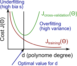
In this section we examine the relationship between the degree of the polynomial d and the underfitting or overfitting of our hypothesis.

We need to distinguish whether bias or variance is the problem contributing to bad predictions.
High bias is underfitting and high variance is overfitting. Ideally, we need to find a golden mean between these two.

The training error will tend to decrease as we increase the degree d of the polynomial.

At the same time, the cross validation error will tend to decrease as we increase d up to a point, and then it will increase as d is increased, forming a convex curve.

High bias (underfitting): both $J\_{train}(\Theta)$ and $J\_{CV}(\Theta)$ will be high. Also, $J\_{CV}(\Theta) \approx J\_{train}(\Theta)$ .

High variance (overfitting): $J\_{train}(\Theta)$ will be low and $J\_{CV}(\Theta)$ will be much greater than $J\_{train}(\Theta)$ .

The is summarized in the figure below:

4. Regularization Bias/Variance

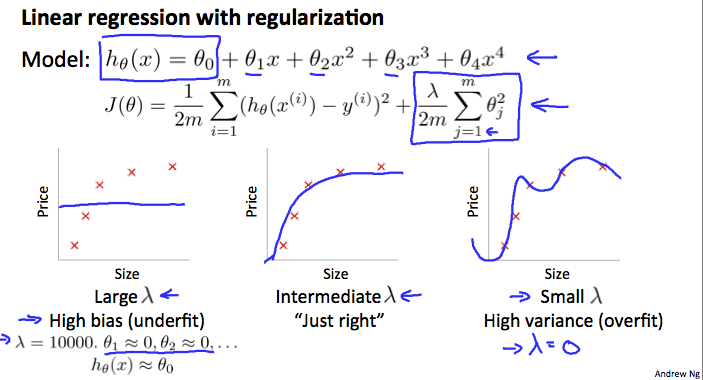
Note: [The regularization term below and through out the video should be $\frac \lambda {2m} \sum\_{j=1}^n \theta\_j ^2$ and NOT $\frac \lambda {2m} \sum\_{j=1}^m \theta\_j ^2$ ]

In the figure above, we see that as λ increases, our fit becomes more rigid. On the other hand, as λ approaches 0, we tend to over overfit the data. So how do we choose our parameter λ to get it ‘just right’ ? In order to choose the model and the regularization term λ, we need to:

Create a list of lambdas (i.e. λ∈{0,0.01,0.02,0.04,0.08,0.16,0.32,0.64,1.28,2.56,5.12,10.24});
Create a set of models with different degrees or any other variants.
Iterate through the λs and for each λ go through all the models to learn some Θ.
Compute the cross validation error using the learned Θ (computed with λ) on the $J\_{CV}(\Theta)$ without regularization or λ = 0. ？？
Select the best combo that produces the lowest error on the cross validation set.
Using the best combo Θ and λ, apply it on $J\_{test}(\Theta)$ to see if it has a good generalization of the problem.

5. Learning Curves

Training an algorithm on a very few number of data points (such as 1, 2 or 3) will easily have 0 errors because we can always find a quadratic curve that touches exactly those number of points. Hence:

As the training set gets larger, the error for a quadratic function increases.
The error value will plateau out after a certain m, or training set size.

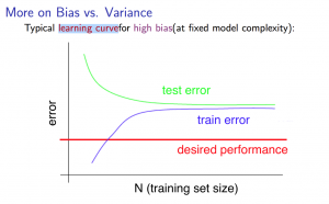
Experiencing high bias:

Low training set size: causes $J\_{train}(\Theta)$ to be low and $J\_{CV}(\Theta)$ to be high.

Large training set size: causes both $J\_{train}(\Theta)$ and $J\_{CV}(\Theta)$ to be high with $J\_{train}(\Theta)$ ≈ $J\_{CV}(\Theta)$ .

If a learning algorithm is suffering from high bias, getting more training data will not (by itself) help much.

me : 随着train sets的增加，高偏差会降低，因为更容易找到合适的 Hypothesis 去拟合数据。所以CV error下降。

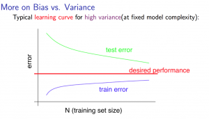
Experiencing high variance:

Low training set size: $J\_{train}(\Theta)$ will be low and $J\_{CV}(\Theta)$ will be high.

Large training set size: $J\_{train}(\Theta)$ increases with training set size and $J\_{CV}(\Theta)$ continues to decrease without leveling off. Also, $J\_{train}(\Theta)$ < $J\_{CV}(\Theta)$ but the difference between them remains significant.

If a learning algorithm is suffering from high variance, getting more training data is likely to help.

me : 随着 train sets 的增加，overfiting 越来越不容易。造成 CV error 下降。

plateau out / leveling off 达到平稳状态
test error will be CV error on picture.

6. What to Do Next Revisited

*Our decision process can be broken down as follows:

Function	Result
Getting more training examples	Fixes high variance
Trying smaller sets of features	Fixes high variance
Increasing λ	Fixes high variance

Adding features	Fixes high bias
Adding polynomial features	Fixes high bias
Decreasing λ	Fixes high bias

6.1 Diagnosing NN

A neural network with fewer parameters is prone to underfitting. It is also computationally cheaper.
A large neural network with more parameters is prone to overfitting. It is also computationally expensive.

In this case you can use regularization (increase λ) to address the overfitting.

6.2 Model Complexity Effects

Lower-order polynomials (low model complexity) have high bias and low variance. In this case, the model fits poorly consistently.
Higher-order polynomials (high model complexity) fit the training data extremely well and the test data extremely poorly. These have low bias on the training data, but very high variance.
In reality, we would want to choose a model somewhere in between, that can generalize well but also fits the data reasonably well.