Coursera Week 3 - Logistic Regression
Logistic Regression
1. Classification
- Email: Spam / Not Spam
- Online Transactions: Fraudulent (Yes/No)?
- Tumor: Malignant / Benign ? [‘tju:mə(r)] [mə’lɪgnənt] / [bɪ’naɪn]
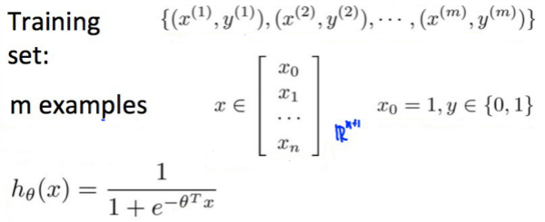
$ y \in {0, 1}$
2. Binary Classification
Instead of our output vector y being a continuous range of values, it will only be 0 or 1.
y∈{0,1}
Where 0 is usually taken as the “negative class” and 1 as the “positive class”, but you are free to assign any representation to it.
Hypothesis Representation
“Sigmoid Function,” also called the “Logistic Function”:
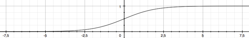
$h_θ$ will give us the probability that our output is 1. For example, $h_θ=0.7$ gives us the probability of 70% that our output is 1.
$
\begin{align}
& h_\theta(x) = P(y=1 | x ; \theta) = 1 - P(y=0 | x ; \theta) \newline& P(y = 0 | x;\theta) + P(y = 1 | x ; \theta) = 1
\end{align}
$
Our probability that our prediction is 0 is just the complement of our probability that it is 1 (e.g. if probability that it is 1 is 70%, then the probability that it is 0 is 30%).
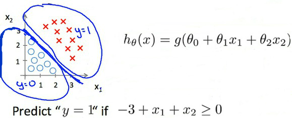
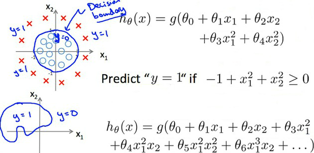
3. Decision Boundary
| Logistic Function | |
|---|---|
| $ \begin{align} & g(z) \geq 0.5 \newline& when \; z \geq 0 \end{align} $ | |
| $ \begin{align} z=0, e^{0}=1 \Rightarrow g(z)=1/2\newline z \to \infty, e^{-\infty} \to 0 \Rightarrow g(z)=1 \newline z \to -\infty, e^{\infty}\to \infty \Rightarrow g(z)=0 \end{align} $ |
| g is $\theta^T X$, then that means: | |
|---|---|
| $ h_\theta(x) = g(\theta^T x) \geq 0.5 $ $ when \; \theta^T x \geq 0 $ | |
| $ \begin{align} & \theta^T x \geq 0 \Rightarrow y = 1 \newline& \theta^T x < 0 \Rightarrow y = 0 \newline \end{align} $ |
The decision boundary is the line that separates the area where y = 0 and where y = 1. It is created by our hypothesis function.
Example:
$
\begin{align}
& \theta = \begin{bmatrix}5 \newline -1 \newline 0\end{bmatrix} \newline & y = 1 \; if \; 5 + (-1) x_1 + 0 x_2 \geq 0 \newline & 5 - x_1 \geq 0 \newline & - x_1 \geq -5 \newline& x_1 \leq 5 \newline \end{align}
$
In this case, our decision boundary is a straight vertical line placed on the graph where $x_1=5$, and everything to the left of that denotes $y = 1$, while everything to the right denotes $y = 0$.
linear decision boundaries
Non-linear decision boundaries
4. Cost Function
We cannot use the same cost function that we use for linear regression because the Logistic Function will cause the output to be wavy, causing many local optima. In other words, it will not be a convex function.
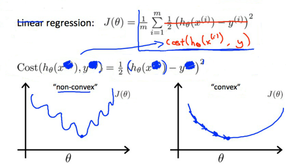
Instead, our cost function for logistic regression looks like:
$
\begin{align}
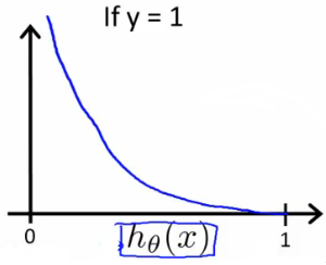
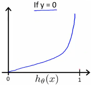
& J(\theta) = \dfrac{1}{m} \sum_{i=1}^m \mathrm{Cost}(h_\theta(x^{(i)}),y^{(i)}) \newline & \mathrm{Cost}(h_\theta(x),y) = -\log(h_\theta(x)) \; & \text{if y = 1} \newline & \mathrm{Cost}(h_\theta(x),y) = -\log(1-h_\theta(x)) \; & \text{if y = 0}
\end{align}
$
$
\begin{align}
& \mathrm{Cost}(h_\theta(x),y) = 0 \text{ if } h_\theta(x) = y \newline & \mathrm{Cost}(h_\theta(x),y) \rightarrow \infty \text{ if } y = 0 \; \mathrm{and} \; h_\theta(x) \rightarrow 1 \newline & \mathrm{Cost}(h_\theta(x),y) \rightarrow \infty \text{ if } y = 1 \; \mathrm{and} \; h_\theta(x) \rightarrow 0 \newline
\end{align}
$
If our correct answer ‘y’ is 0, then the cost function will be 0 if our hypothesis function also outputs 0. If our hypothesis approaches 1, then the cost function will approach infinity.
If our correct answer ‘y’ is 1, then the cost function will be 0 if our hypothesis function outputs 1. If our hypothesis approaches 0, then the cost function will approach infinity.
5. Cost Function & Gradient Desc
We can compress our cost function's two conditional cases into one case:
$ \mathrm{Cost}(h_\theta(x),y) = - y \cdot \log(h_\theta(x)) - (1 - y) \cdot \log(1 - h_\theta(x))$
We can fully write out our entire cost function as follows:
$
J(\theta) = - \frac{1}{m} \displaystyle \sum_{i=1}^m [y^{(i)}\log (h_\theta (x^{(i)})) + (1 - y^{(i)})\log (1 - h_\theta(x^{(i)}))]
$
A vectorized implementation is:
$
\begin{align}
& h = g(X\theta)\newline
& J(\theta) = \frac{1}{m} \cdot \left(-y^{T}\log(h)-(1-y)^{T}\log(1-h)\right)
\end{align}
$
5.1 Gradient Descent
Remember that the general form of gradient descent is:
$
\begin{align}
& Repeat \; \lbrace \newline & \; \theta_j := \theta_j - \alpha \dfrac{\partial}{\partial \theta_j}J(\theta) \newline & \rbrace
\end{align}
$
We can work out the derivative part using calculus to get:
$
\begin{align}
& Repeat \; \lbrace \newline
& \; \theta_j := \theta_j - \frac{\alpha}{m} \sum_{i=1}^m (h_\theta(x^{(i)}) - y^{(i)}) x_j^{(i)} \newline & \rbrace
\end{align}
$
seen 5.2 detailed
A vectorized implementation is:
$
\theta := \theta - \frac{\alpha}{m} X^{T} (g(X \theta ) - \vec{y})
$
5.2 Partial derivative of J(θ)
partial [‘pɑːʃ(ə)l]
derivative [dɪ’rɪvətɪv]
$
\begin{align}
\sigma(x)’&=\left(\frac{1}{1+e^{-x}}\right)’=\frac{-(1+e^{-x})’}{(1+e^{-x})^2}=\frac{-1’-(e^{-x})’}{(1+e^{-x})^2}=\frac{0-(-x)’(e^{-x})}{(1+e^{-x})^2}=\frac{-(-1)(e^{-x})}{(1+e^{-x})^2}=\frac{e^{-x}}{(1+e^{-x})^2} \newline &=\left(\frac{1}{1+e^{-x}}\right)\left(\frac{e^{-x}}{1+e^{-x}}\right)=\sigma(x)\left(\frac{+1-1 + e^{-x}}{1+e^{-x}}\right)=\sigma(x)\left(\frac{1 + e^{-x}}{1+e^{-x}} - \frac{1}{1+e^{-x}}\right)=\sigma(x)(1 - \sigma(x))
\end{align}
$
Now we are ready to find out resulting partial derivative:
$
\begin{align}
\frac{\partial}{\partial \theta_j} J(\theta) &= \frac{\partial}{\partial \theta_j} \frac{-1}{m}\sum_{i=1}^m \left [ y^{(i)} log (h_\theta(x^{(i)})) + (1-y^{(i)}) log (1 - h_\theta(x^{(i)})) \right ] \newline&= - \frac{1}{m}\sum_{i=1}^m \left [ y^{(i)} \frac{\partial}{\partial \theta_j} log (h_\theta(x^{(i)})) + (1-y^{(i)}) \frac{\partial}{\partial \theta_j} log (1 - h_\theta(x^{(i)}))\right ] \newline&= - \frac{1}{m}\sum_{i=1}^m \left [ \frac{y^{(i)} \frac{\partial}{\partial \theta_j} h_\theta(x^{(i)})}{h_\theta(x^{(i)})} + \frac{(1-y^{(i)})\frac{\partial}{\partial \theta_j} (1 - h_\theta(x^{(i)}))}{1 - h_\theta(x^{(i)})}\right ] \newline&= - \frac{1}{m}\sum_{i=1}^m \left [ \frac{y^{(i)} \frac{\partial}{\partial \theta_j} \sigma(\theta^T x^{(i)})}{h_\theta(x^{(i)})} + \frac{(1-y^{(i)})\frac{\partial}{\partial \theta_j} (1 - \sigma(\theta^T x^{(i)}))}{1 - h_\theta(x^{(i)})}\right ] \newline&= - \frac{1}{m}\sum_{i=1}^m \left [ \frac{y^{(i)} \sigma(\theta^T x^{(i)}) (1 - \sigma(\theta^T x^{(i)})) \frac{\partial}{\partial \theta_j} \theta^T x^{(i)}}{h_\theta(x^{(i)})} + \frac{- (1-y^{(i)}) \sigma(\theta^T x^{(i)}) (1 - \sigma(\theta^T x^{(i)})) \frac{\partial}{\partial \theta_j} \theta^T x^{(i)}}{1 - h_\theta(x^{(i)})}\right ] \newline&= - \frac{1}{m}\sum_{i=1}^m \left [ \frac{y^{(i)} h_\theta(x^{(i)}) (1 - h_\theta(x^{(i)})) \frac{\partial}{\partial \theta_j} \theta^T x^{(i)}}{h_\theta(x^{(i)})} - \frac{(1-y^{(i)}) h_\theta(x^{(i)}) (1 - h_\theta(x^{(i)})) \frac{\partial}{\partial \theta_j} \theta^T x^{(i)}}{1 - h_\theta(x^{(i)})}\right ] \newline&= - \frac{1}{m}\sum_{i=1}^m \left [ y^{(i)} (1 - h_\theta(x^{(i)})) x^{(i)}_j - (1-y^{(i)}) h_\theta(x^{(i)}) x^{(i)}_j\right ] \newline&= - \frac{1}{m}\sum_{i=1}^m \left [ y^{(i)} (1 - h_\theta(x^{(i)})) - (1-y^{(i)}) h_\theta(x^{(i)}) \right ] x^{(i)}_j \newline&= - \frac{1}{m}\sum_{i=1}^m \left [ y^{(i)} - y^{(i)} h_\theta(x^{(i)}) - h_\theta(x^{(i)}) + y^{(i)} h_\theta(x^{(i)}) \right ] x^{(i)}_j \newline&= - \frac{1}{m}\sum_{i=1}^m \left [ y^{(i)} - h_\theta(x^{(i)}) \right ] x^{(i)}_j \newline&= \frac{1}{m}\sum_{i=1}^m \left [ h_\theta(x^{(i)}) - y^{(i)} \right ] x^{(i)}_j
\end{align}
$
The vectorized version;
$
\nabla J(\theta) = \frac{1}{m} \cdot X^T \cdot \left(g\left(X\cdot\theta\right) - \vec{y}\right)
$
6. Advanced Optimization
We can apply regularization to both linear regression and logistic regression. We will approach linear regression first.
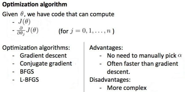
We first need to provide a function that evaluates the following two functions for a given input value θ:
$
\begin{align}
& J(\theta) \newline & \dfrac{\partial}{\partial \theta_j}J(\theta)
\end{align}
$
We can write a single function that returns both of these…
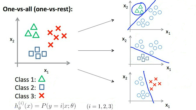
7. Multiclass Classification
$
\begin{align}
& y \in \lbrace0, 1 … n\rbrace \newline& h_\theta^{(0)}(x) = P(y = 0 | x ; \theta) \newline& h_\theta^{(1)}(x) = P(y = 1 | x ; \theta) \newline& \cdots \newline& h_\theta^{(n)}(x) = P(y = n | x ; \theta) \newline& \mathrm{prediction} = \max_i( h_\theta ^{(i)}(x) )\newline
\end{align}
$
Train a logistic regression classifier $h_\theta ^{(i)}(x)$ for each class $i$ to predict the probability that $y = i$ .
On a new input $x$, to make a prediction, pick the $i$ class that maximizes $\max_i( h_\theta ^{(i)}(x)$
@2017-02-10 review done.
8. Regularization
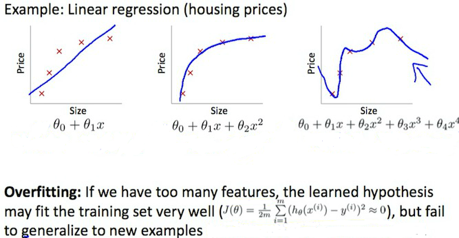
The Problem of Overfitting
Regularization is designed to address the problem of overfitting.
High bias or underfitting is when the form of our hypothesis function h maps poorly to the trend of the data. It is usually caused by a function that is too simple or uses too few features.
eg. if we take $h_θ(x)=θ_0+θ_1 \cdot x_1+θ_2 \cdot x_2$ then we are making an initial assumption that a linear model will fit the training data well and will be able to generalize but that may not be the case.
At the other extreme, overfitting or high variance is caused by a hypothesis function that fits the available data but does not generalize well to predict new data. It is usually caused by a complicated function that creates a lot of unnecessary curves and angles unrelated to the data.
This terminology is applied to both linear and logistic regression. There are two main options to address the issue of overfitting:
1) Reduce the number of features:
a) Manually select which features to keep.
b) Use a model selection algorithm .
2) Regularization
- Keep all the features, but reduce the parameters $θ_j$.
Regularization works well when we have a lot of slightly useful features.
to address 提出,去解决
9. Regularization Cost Function
If we have overfitting from our hypothesis function, we can reduce the weight that some of the terms in our function carry by increasing their cost.
Say we wanted to make the following function more quadratic [kwɒ’drætɪk]:
$
\theta_0 + \theta_1x + \theta_2x^2 + \theta_3x^3 + \theta_4x^4
$
We’ll want to eliminate the influence of $\theta_3x^3$ and $\theta_4x^4$. Without actually getting rid of these features or changing the form of our hypothesis, we can instead modify our cost function:
$
min_\theta\ \dfrac{1}{2m}\sum_{i=1}^m (h_\theta(x^{(i)}) - y^{(i)})^2 + 1000 \cdot \theta_3^2 + 1000\cdot\theta_4^2
$
We’ve added two extra terms at the end to inflate the cost of $\theta_3$ and $\theta_4$. Now, in order for the cost function to get close to zero, we will have to reduce the values of $\theta_3$ and $\theta_4$ to near zero. This will in turn greatly reduce the values of $\theta_3x^3$ and $\theta_4x^4$ in our hypothesis function.
We could also regularize all of our theta parameters in a single summation:
$
min_\theta\ \dfrac{1}{2m}\ \left[ \sum_{i=1}^m (h_\theta(x^{(i)}) - y^{(i)})^2 + \lambda\ \sum_{j=1}^n \theta_j^2 \right]
$
The λ, or lambda, is the regularization parameter. It determines how much the costs of our theta parameters are inflated.
You can visualize the effect of regularization in this interactive plot : https://www.desmos.com/calculator/1hexc8ntqp
Using the above cost function with the extra summation, we can smooth the output of our hypothesis function to reduce overfitting. If lambda is chosen to be too large, it may smooth out the function too much and cause underfitting.
我们可以平滑我们的假设函数的输出,以减少过度拟合
10. Regularized Linear
10.1 Gradient Descent
$
\begin{align}
& \text{Repeat}\ \lbrace \newline
& \ \ \ \ \theta_0 := \theta_0 - \alpha\ \frac{1}{m}\ \sum_{i=1}^m (h_\theta(x^{(i)}) - y^{(i)})x_0^{(i)} \newline
& \ \ \ \ \theta_j := \theta_j - \alpha\ \left[ \left( \frac{1}{m}\ \sum_{i=1}^m (h_\theta(x^{(i)}) - y^{(i)})x_j^{(i)} \right) + \frac{\lambda}{m}\theta_j \right] &\ \ \ \ \ \ \ \ \ \ j \in \lbrace 1,2…n\rbrace\newline
& \rbrace
\end{align}
$
The term $\frac{\lambda}{m}\theta_j$ performs our regularization.
$
\theta_j := \theta_j(1 - \alpha\frac{\lambda}{m}) - \alpha\frac{1}{m}\sum_{i=1}^m(h_\theta(x^{(i)}) - y^{(i)})x_j^{(i)}
$
The first term in the above equation, $1 - \alpha\frac{\lambda}{m}$ will always be less than 1. Intuitively you can see it as reducing the value of $\theta_j$ by some amount on every update.
10.2 Normal Equation
Use less, temporarily ignored
11. Regularized Logistic
Cost Function
$
J(\theta) = - \frac{1}{m} \sum_{i=1}^m \large[ y^{(i)}\ \log (h_\theta (x^{(i)})) + (1 - y^{(i)})\ \log (1 - h_\theta(x^{(i)})) \large]
$
We can regularize this equation by adding a term to the end:
$
J(\theta) = - \frac{1}{m} \sum_{i=1}^m \large[ y^{(i)}\ \log (h_\theta (x^{(i)})) + (1 - y^{(i)})\ \log (1 - h_\theta(x^{(i)}))\large] + \frac{\lambda}{2m}\sum_{j=1}^n \theta_j^2
$
Gradient Descent
Just like with linear regression, we will want to separately update $\theta_0$ and the rest of the parameters because we do not want to regularize $\theta_0$.
$
\begin{align}
& \text{Repeat}\ \lbrace \newline& \ \ \ \ \theta_0 := \theta_0 - \alpha\ \frac{1}{m}\ \sum_{i=1}^m (h_\theta(x^{(i)}) - y^{(i)})x_0^{(i)} \newline& \ \ \ \ \theta_j := \theta_j - \alpha\ \left[ \left( \frac{1}{m}\ \sum_{i=1}^m (h_\theta(x^{(i)}) - y^{(i)})x_j^{(i)} \right) + \frac{\lambda}{m}\theta_j \right] &\ \ \ \ \ \ \ \ \ \ j \in \lbrace 1,2…n\rbrace\newline& \rbrace\end{align}
$
Reference article
Going to a restaurant L2 Arriving at a restaurant
1. Vocabulary mushroom soup Caesar salad fresh oysters shrimp cocktail roasted chicken with veget...
Going to a restaurant L1 Making a restaurant reservation
1. Vocabulary specialty authentic reputation reviews a wide variety of [və’raɪətɪ] choices free ...
Checking if Disqus is accessible...