%% Change Octave prompt PS1('>> '); %% Change working directory in windows example: cd 'c:/path/to/desired/directory name' %% Note that it uses normal slashes and does not use escape characters for the empty spaces.
%% variable assignment a = 3; % semicolon suppresses output b = 'hi'; c = 3>=1;
% Displaying them: a = pi disp(a) disp(sprintf('2 decimals: %0.2f', a)) disp(sprintf('6 decimals: %0.6f', a)) format long a format short a
%% vectors and matrices A = [12; 34; 56]
v = [123] v = [1; 2; 3] v = 1:0.1:2% from 1 to 2, with stepsize of 0.1. Useful for plot axes v = 1:6% from 1 to 6, assumes stepsize of 1 (row vector)
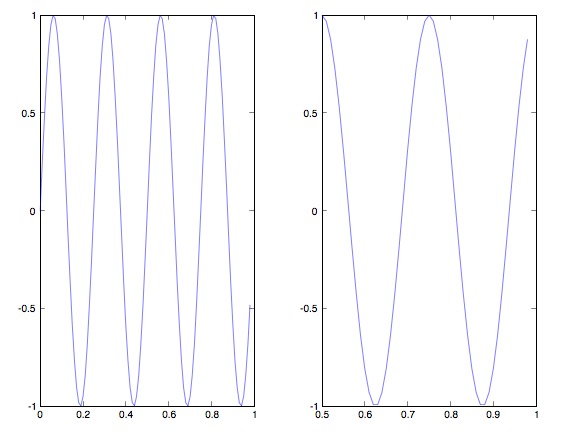
C = 2*ones(2,3) % same as C = [2 2 2; 2 2 2] w = ones(1,3) % 1x3 vector of ones w = zeros(1,3) w = rand(1,3) % drawn from a uniform distribution w = randn(1,3)% drawn from a normal distribution (mean=0, var=1) w = -6 + sqrt(10)*(randn(1,10000)); % (mean = -6, var = 10) - note: add the semicolon hist(w) % plot histogram using 10 bins (default) hist(w,50) % plot histogram using 50 bins % note: if hist() crashes, try "graphics_toolkit('gnu_plot')"
%% dimensions sz = size(A) % 1x2 matrix: [(number of rows) (number of columns)] size(A,1) % number of rows size(A,2) % number of cols length(v) % size of longest dimension
%% loading data pwd % show current directory (current path) cd 'C:\Users\ang\Octave files'% change directory ls % list files in current directory load q1y.dat % alternatively, load('q1y.dat') load q1x.dat who % list variables in workspace whos % list variables in workspace (detailed view) clear q1y % clear command without any args clears all vars v = q1x(1:10); % first 10 elements of q1x (counts down the columns) save hello.mat v; % save variable v into file hello.mat save hello.txt v -ascii; % save as ascii % fopen, fread, fprintf, fscanf also work [[not needed in class]]
%% indexing A(3,2) % indexing is (row,col) A(2,:) % get the 2nd row. % ":" means every element along that dimension A(:,2) % get the 2nd col A([13],:) % print all the elements of rows 1 and 3
A(:,2) = [10; 11; 12] % change second column A = [A, [100; 101; 102]]; % append column vec A(:) % Select all elements as a column vector.
% Putting data together A = [12; 34; 56] B = [1112; 1314; 1516] % same dims as A C = [A B] % concatenating A and B matrices side by side C = [A, B] % concatenating A and B matrices side by side C = [A; B] % Concatenating A and B top and bottom
%% initialize variables A = [12;34;56] B = [1112;1314;1516] C = [11;22] v = [1;2;3]
%% matrix operations A * C % matrix multiplication A .* B % element-wise multiplication % A .* C or A * B gives error - wrong dimensions A .^ 2% element-wise square of each element in A 1./v % element-wise reciprocal log(v) % functions like this operate element-wise on vecs or matrices exp(v) abs(v)
-v % -1*v
v + ones(length(v), 1) % v + 1 % same
A' % matrix transpose
%% misc useful functions
% max (or min) a = [11520.5] val = max(a) [val,ind] = max(a) % val - maximum element of the vector a and index - index value where maximum occur val = max(A) % if A is matrix, returns max from each column
% compare values in a matrix & find a < 3% checks which values in a are less than 3 find(a < 3) % gives location of elements less than 3 A = magic(3) % generates a magic matrix - not much used in ML algorithms [r,c] = find(A>=7) % row, column indices for values matching comparison
% sum, prod sum(a) prod(a) floor(a) % or ceil(a) max(rand(3),rand(3)) max(A,[],1) - maximum along columns(defaults to columns - max(A,[])) max(A,[],2) - maximum along rows A = magic(9) sum(A,1) sum(A,2) sum(sum( A .* eye(9) )) sum(sum( A .* flipud(eye(9)) ))
>> i = 1; >> whilei <= 5, v(i) = 100; i = i+1; end; >> v v =
100 100 100 100 100 64 128 256 512 1024
>> i = 1; >> whiletrue, v(i) = 999; i = i + 1; ifi == 6, break; end; end; >> v v =
999 999 999 999 999 64 128 256 512 1024 >> v(1) ans = 999 >> v(1) = 2; >> if v(1) == 1, disp('The value is one'); elseif v(1) == 2, disp('The value is two'); else disp('The value is not 1 or 2'); end; The value is two
6. Functions
To call the function in Octave, do either:
Navigate to the directory of the functionName.m file and call the function:
>> (1^2 + 2^2 + 3^2) / (2*3)
ans =  2.3333
>> [-1,-2,-3]*[-1;-2;-3]
ans =  14
>> 14 / 6
ans =  2.3333
>>
7. Vectorization
Vectorization is the process of taking code that relies on loops and converting it into matrix operations. It is more efficient, more elegant, and more concise.
As an example, let’s compute our prediction from a hypothesis. Theta is the vector of fields for the hypothesis and x is a vector of variables.
Checking if Disqus is accessible...